A GAIN-SCHEDULING APPROACH FOR

AIRSHIP PATH-TRACKING

Alexandra Moutinho

IDMEC - IST

Instituto Superior T

ecnico, Av. Rovisco Pais, 1047-001 Lisbon, Portugal

Jos

e Raul Azinheira

IDMEC - IST

Instituto Superior T

ecnico, Av. Rovisco Pais, 1047-001 Lisbon, Portugal

Keywords:

UAV, gain-scheduling, path-tracking, optimal control, airship.

Abstract:

In this paper a gain scheduled optimal controller is designed to solve the path-tracking problem of an airship.

The control law is obtained from a coupled linear model of the airship that allows to control the longitudinal

and lateral motions simultaneously. Due to the importance of taking into account wind effects, which are

rather important due to the airship large volume, the wind is included in the kinematics, and the dynamics

is expressed as function of the air velocity. Two examples are presented with the inclusion of wind, one

considering a constant wind input and the other considering in addition a 3D turbulent gust, demonstrating the

effectiveness of this single controller tracking a reference path over the entire ﬂight envelope.

1 INTRODUCTION

The range of civilian and military applications of Un-

manned Aerial Vehicles (UAV’s) is driving the growth

of the rapidly changing market for UAVs globally.

The list of applications and opportunities in this do-

main is already large and is continually growing.

Among these are inspection oriented applications that

cover different areas such as mineral and archaeo-

logic prospecting, land use surveys in rural and urban

regions, inspection of man-made structures such as

pipelines, power transmission lines, dams and roads.

Most of the applications cited above have proﬁles

that require maneuverable low altitude, low speed air-

borne data gathering platforms. The vehicle should

also be able to hover above an observation target,

present extended airborne capabilities for long dura-

tion studies, take-off and land vertically without the

need of runway infrastructures, have a large payload

to weight ratio, among other requisites. For this sce-

nario, lighter-than-air (LTA) vehicles, like airships,

are often better suited than balloons, airplanes and he-

licopters (Elfes et al., 1998), mainly because: they de-

rive the largest part of their lift from aerostatic, rather

than aerodynamic forces; they are safer and, in case

of failure, present a graceful degradation; they are in-

trinsically of higher stability than other platforms.

For all its advantages, airships are being chosen

as platform to a variety of applications. Some ex-

amples are demining

, ﬁre detection (Merino et al.,

2005), emergency management (Rao et al., 2005), tar-

get search (Xia and Corbett, 2005) and even explo-

ration of planetary bodies (Elfes et al., 2003).

In some cases, the airship is remotely maneuvered,

but a wider range of applications is achievable with

unmanned autonomous airships, which requires an ef-

fective control of the robot behavior. Like other aerial

vehicles, the airship dynamics is highly nonlinear. It

mostly varies with the relative airspeed, which inﬂu-

ences both acting forces as well as actuators authority.

In ﬂight control design, it is an established practice to

base the controller design in a linear description of

the system, obtained assuming the motion of the aer-

ial vehicle is constrained to small perturbations about

a trimmed equilibrium ﬂight condition (Stevens and

Lewis, 1992). For instance, Hygounenc and Sou

eres

consider linear decoupled models for the longitudinal

and lateral motions. The vertical movement is reg-

ulated using a Lyapunov based approach, while the

horizontal path-following problem is independently

solved with a PI controller (Hygounenc and Sou

eres,

2003). Xia and Corbett apply the slidding mode tech-

nique to the linear decoupled systems in order to ob-

tain a cooperative control system for two blimps (Xia

and Corbett, 2005). Complementing the linear model

of the airship with the vector of visual signals, Sil-

veira et al. report a line following visual servo control

www.mineseeker.com

Moutinho A. and Azinheira J. (2006).

A GAIN-SCHEDULING APPROACH FOR AIRSHIP PATH-TRACKING.

In Proceedings of the Third International Conference on Informatics in Control, Automation and Robotics, pages 82-88

DOI: 10.5220/0001219800820088

 SciTePress

scheme with a PID structure (Silveira et al., 2003).

Although using different control methodologies,

the above references all implicitly use the gain

scheduling approach (

Astr

om and Wittenmark, 1989;

Khalil, 2000a), the prevailing ﬂight control design

methodology nowadays (Rugh and Shamma, 2000).

As mentioned, the linear model of the system is an ap-

proximation only valid for small perturbations around

an equilibrium condition, which leads to the necessity

of repeating the linearization process for several trim

points over the desired operation range.

In this paper a gain scheduled optimal controller is

designed to solve the path-tracking problem for the

airship of the Aurora (Autonomous Unmanned Re-

mote mOnitoring Robotic Airship) project (de Paiva

et al., 2006). The control law is obtained from a cou-

pled linear model of the airship that allows to control

the longitudinal and lateral motions simultaneously.

Due to the importance of taking into account wind ef-

fects, which are rather important due to the airship

large volume, the wind is included in the kinemat-

ics, and the dynamics is expressed as function of the

air velocity. The designed controller has been tested

exhaustively in simulation environment prior to real

implementation, and effective results have been ob-

tained covering the entire ﬂight envelope with the sin-

gle controller. We present here two cases concern-

ing the same reference tracking: a nominal case and

a case considering realistic wind disturbances, which

the airship platform is supposed to face during its nor-

mal operation.

In this article we start by describing the Aurora air-

ship platform, followed by the deﬁnition of the model

used in the control design (§ 2). In § 4 we propose an

optimal gain scheduled control, applied to the path-

tracking problem in § 3. So as to illustrate the valu-

able results obtained, in § 5 we show examples of the

proposed control acting over the entire ﬂight envelope

in the presence of wind disturbances. Finally, conclu-

sions are summarized in § 6.

2 AIRSHIP DESCRIPTION

2.1 Airship Platform

In this section we brieﬂy describe the airship platform

of the Aurora project (de Paiva et al., 2006).

The LTA robotic prototype has been built as an evo-

lution of the Airspeed Airships’ AS800. It is a non-

rigid airship with 10.5m long, 3.0m diameter, and

34m

of volume, whose payload capacity is approxi-

mately 10kg and maximum speed is around 50km/h

(see ﬁg. 1). As main control actuators, the airship has:

i) four deﬂection surfaces at the tail in the ’×’ con-

ﬁguration; ii) the thrust provided by two propellers

driven by two-stroke engines; iii) the vectoring of this

propulsion group.

Figure 1: The Aurora airship.

The airship system state variables are measured by

a GPS with differential correction, an inertial mea-

surement unit and a wind sensor.

2.2 Airship Model

Consider an underactuated airship modeled as a rigid

body subject to forces and torques. Let {i} repre-

sent the inertial frame (which, for simplicity, is con-

sidered coincident with the geographical north-east-

down (NED) frame), {l} be the body-ﬁxed coordinate

frame whose origin is located in the airship center of

volume, and S(Φ) ∈ SO(3) := {S ∈ R

3×3

: SS

′

I, det(S) = +1} is the rotation matrix from {i} to

{l} frame, and where Φ ∈ R

3×1

is the attitude of {l}

in relation to {i} expressed as the Euler angles roll φ,

pitch θ and yaw ψ.

The airship dynamic equations of motion (Azin-

heira et al., 2002) may be condensed in the form

V = −Ω

MV + ESg + F

+ f(U

, V

) (1)

P = JV (2)

where V = [v

′

, ω

′

]

′

∈ R

6×1

includes the airship lin-

ear and angular velocities relative to {i} expressed in

{l}, P = [p

′

, Φ

′

]

′

∈ R

6×1

contains the airship carte-

sian and angular positions expressed in the {i} frame,

J = diag{S

′

, R} ∈ R

6×6

, R = R(Φ) ∈ R

3×3

is a

coefﬁcient matrix, and M ∈ R

6×6

is the symmetric

inertia matrix. Ω

= diag{Ω(ω), Ω(ω)} ∈ R

6×6

Ω(ω) ∈ R

3×3

is the skew-symmetric matrix equiva-

lent to the cross-product ω×, E ∈ R

6×3

is the gravity

matrix input, and g ∈ R

3×1

represents the gravity ac-

celeration in the {i} frame. F

∈ R

6×1

stands for the

aerodynamic forces and moments.

The input forces and torques f(U

, V

) ∈ R

6×1

are

a nonlinear function of the airship airspeed V

and of

the actuators input U

∈ R

6×1

, which includes the

elevator δ

, the total left and right engines thrust X

the engines vectoring angle δ

, and the rudder δ

(see

ﬁgure 2).

A GAIN-SCHEDULING APPROACH FOR AIRSHIP PATH-TRACKING

−

Figure 2: Airship actuators.

2.2.1 Inclusion of Wind

We assume that the inertial wind velocity vector

= S

′

is constant over a region much larger

than the size of the airship. This means we do not

consider wind shearing effects and torques exerted on

the airship (ω

= 0).

The velocity of the airship center of volume with

respect to the air represented in the {l} frame is given

= v − v

(3)

In order to include the wind inﬂuence in the airship

equations of motion, the wind components must be

supplied as inputs. Then v

, rather than v, must be

used in the calculation of the aerodynamic forces and

moments. The airship dynamics and kinematics can

then be rewritten as

= M

−1

[−Ω

+ ESg + F

+ f(U

)]

(4)

P = JV

+ S

′

(5)

with V

= [v

′

, ω

′

]

′

and V

= [v

′

, 0]

′

As mentioned before, the wind must be provided

as input to equations (4) and (5). Since the wind is

not directly measurable, we will need to compute an

estimate. Knowing that

cos(α) cos(β)

sin(β)

sin(α) cos(β)

(6)

where the airspeed V

, the angle of attack α and the

sideslip angle β are measurable quantities, we can

compute the wind velocity vector v

using equation

(3).

2.2.2 Linear Model

The complexity of the nonlinear dynamic equations

justiﬁes the search for a linear simpliﬁed version, also

necessary if to use the gain-scheduling approach.

The linearization of the dynamic equations (4)-(5)

is made for trimmed conditions around equilibrium,

which is commonly an horizontal straight ﬂight, with-

out wind incidence.

Considering only the dynamic or perturbed part,

and for the conditions stated, the motion equations

are written for a perturbation vector x of the states

around the equilibrium value X

, and the perturbed

input u around the trimmed value U

, resulting in the

matricial dynamic equation:

x = Ax + Bu (7)

in the absence of disturbances (deterministic case).

The linearized model (7), i.e., the dynamic and in-

put matrices A and B, depend on the trim point cho-

sen for the linearization, and in particular of the cho-

sen airspeed V

(we consider here low altitude ﬂight,

where the altitude variation is insufﬁcient to signiﬁ-

cantly change the envelope pressure). The existence

of a constant wind component is also to be consid-

ered.

In ﬂight control, and as a result of the applica-

tion of the small perturbations theory, two indepen-

dent (decoupled) linear models are usually obtained,

corresponding to the lateral and longitudinal mo-

tions (Stevens and Lewis, 1992). Here, we chose to

work with a single linear model, which allows us to

design a single controller for the lateral and longitu-

dinal movements.

Considering that all variables now correspond to

the perturbation term, the state and input vectors of

the dynamics equation (7) are x = [v

′

, ω

′

, p

′

, Φ

′

]

′

and u = [δ

, X

, δ

]

′

3 PATH-TRACKING PROBLEM

Let us start by deﬁne the vehicle mission: to force the

output to follow a reference signal, a given function

of time, and to drive to zero the tracking error:

e(t) = y(t) − y

(t) (8)

This path-tracking problem differs from the path-

following one by the fact that the path reference is

time dependent.

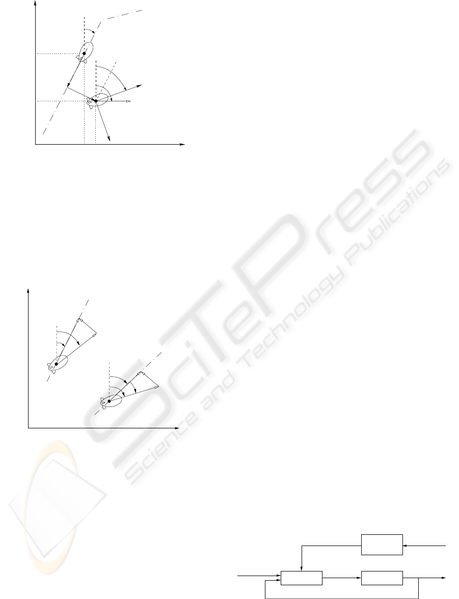
We deﬁne here the cartesian position error e

[η, δ, γ]

′

as expressed in the reference path frame and

computed by (see ﬁg. 3)

= S(Φ

)(p − p

) (9)

The reference path attitude Φ

= [φ

, θ

, ψ

]

′

obtained considering φ

= 0, and θ

and ψ

as the

angles the reference trajectory does respectively with

the horizontal plane, and the north direction.

The attitude error is the difference between the air-

ship and reference attitudes:

= Φ − Φ

(10)

ICINCO 2006 - ROBOTICS AND AUTOMATION

E y

reference

path

Figure 3: Position errors deﬁnition (2D).

If we were not taking into account the wind input,

≡ Φ

. However, due to the sideslip, the airship

orients itself with the relative air direction (see ﬁg. 4).

Therefore, the attitude reference Φ

corresponds to

the estimated attitude of the reference velocity inﬂu-

enced by the wind,

reference

position

actual

Figure 4: Reference heading estimation (2D).

We compute the reference attitude Φ

following

these three steps:

1. with the airship inertial velocity

p, its attitude Φ

and the aerodynamic variables V

, β and α (all

measured variables), estimate the wind inertial ve-

locity vector

using equations (6) and (3), and

knowing that

p = S(Φ)

′

2. compute the velocity in the aerodynamic frame

as the inertial vectors difference between the air-

ship reference velocity

and the wind velocity

estimation

;

3. consider φ

= 0, and θ

and ψ

as the angles

does respectively with the horizontal plane,

and the north direction.

The objective of the control design proposed in the

next section is then to drive to zero the errors given by

equations (9) and (10).

4 GAIN-SCHEDULING

The linearized system model (7) presented before is

only valid for small regions around trim conditions.

This reveals the basic limitation of the design via the

linearization approach, the fact that the controller is

guaranteed to work only in the neighborhood of a sin-

gle operating (equilibrium) point. The gain schedul-

ing technique (Khalil, 2000b) addressed here allows

to extend the validity of the linearization approach to

a range of operating points, in this case over the entire

ﬂight envelope.

It is sometimes possible to ﬁnd auxiliary variables

that correlate well with the changes in the process dy-

namics. In the airship case, these variables mostly

correspond to the airspeed V

and altitude h. Still, the

altitude inﬂuence may be disregarded for low altitude

ﬂights where the envelope pressure is kept practically

constant. The airspeed, however, has a major inﬂu-

ence over the airship behavior. It not only determines

the magnitude of the aerodynamic forces acting on

the airship, but also rules the inﬂuence of the actua-

tors on the airship motion. As example, the action of

the control surfaces, corresponding to the standard in-

puts δ

and δ

, is a function of the dynamic pressure

and varies as the square of the airspeed (Stevens and

Lewis, 1992), which leads to a reduced authority of

these actuators when ﬂying at low airspeeds.

Obtaining a linearized system at several equilib-

rium points, followed by the design of a linear feed-

back controller for each point, and implementation of

the resulting family of linear controllers as a single

controller whose parameters are changed by monitor-

ing the scheduling variable, results in a gain sched-

uled controller (see ﬁgure 5). This controller is ex-

pected to maintain the stability and performance of

the linear systems as long as the design models are

reasonable representations of the system dynamics

and as long as the scheduling variable varies ”slowly”.

command

output

u y

signal

regulator

control

process

gain

schedule

regulator

parameters

operating

condition

signal

Figure 5: Gain-scheduling block diagram.

A GAIN-SCHEDULING APPROACH FOR AIRSHIP PATH-TRACKING

4.1 Optimal Control

Here we discuss the design of a servo control sys-

tem whose purpose is to keep the tracking error small,

while the airship ﬂight condition is kept near the equi-

librium state.

Consider the linear system deﬁned by equation (7),

assume the complete state x is measurable, and that

the output variable

y = Cx (11)

is to track a reference input y

. The tracking error is

then deﬁned as

e = y − y

(12)

Considering that the model represents the deviations

from an equilibrium state X

, it is required that the

state variables x

that do not form the output vector

be kept null, in order to have X

= X

The admissible control is a proportional output

feedback of the form

u = K

e − K

= −Kz (13)

where z = [e

′

, x

′

]

′

and K = [K

We use an optimal Linear Quadratic regulator to

obtain the control effort (13), that results from the

minimization of the cost function

J =

∞

′

Qz + u

′

Ru)dt (14)

subject to the system dynamics (7). The state and con-

trol weighting matrices Q ≥ 0 and R > 0 are the

designer tools to balance the state errors z against the

control effort u. In the airship control case, the con-

trol weighting matrix R is a specially important tool

in the sense that it allows the designer to change the

control effort of the different actuators over the ﬂight

envelope.

The gain matrix K is obtained from

K = R

−1

′

P (15)

solving ﬁrst the algebraic Riccati equation for the pos-

itive deﬁnite matrix P

PA + A

′

P − PBR

−1

′

P + Q = 0 (16)

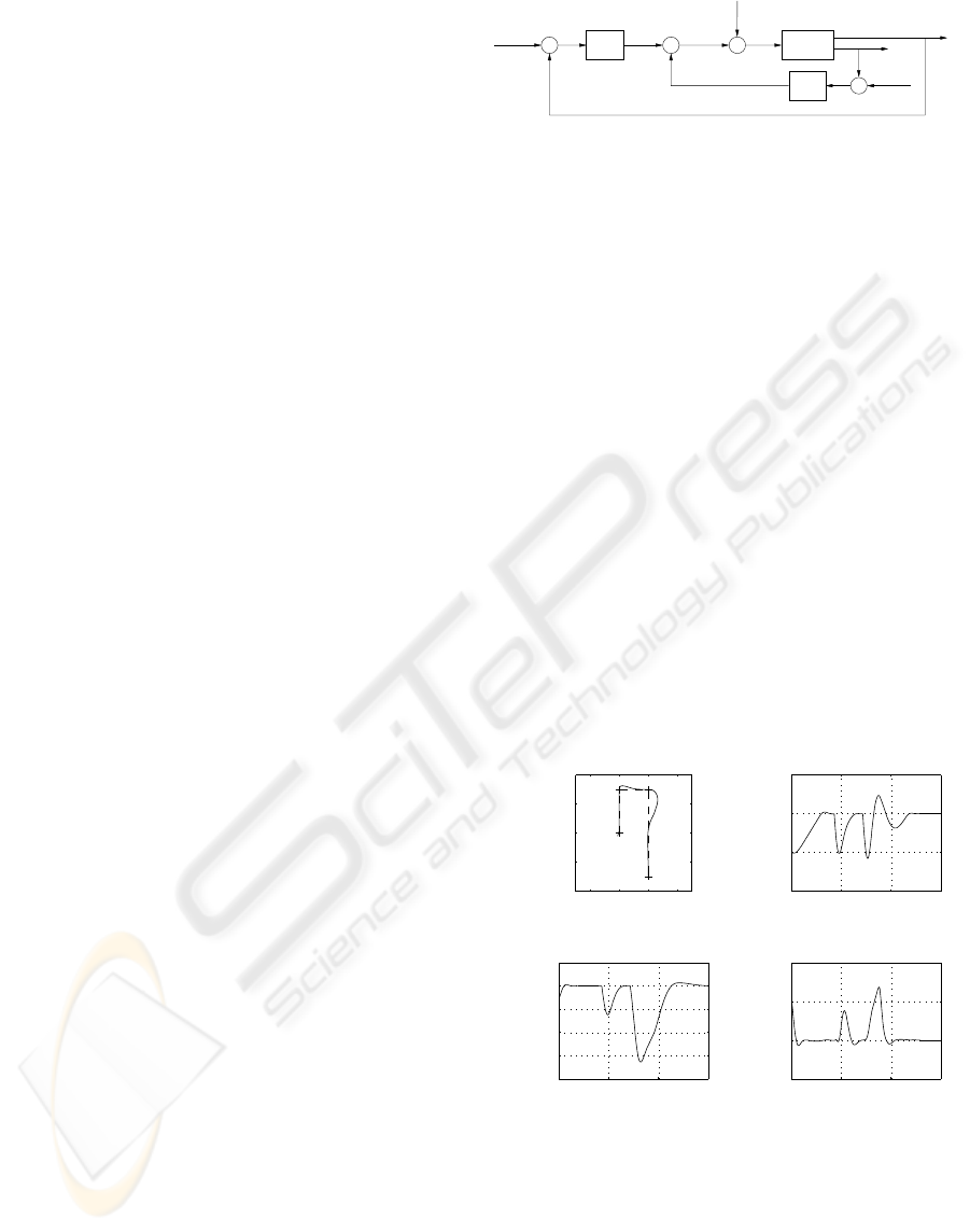
The actuators request

U = U

+ u (17)

has to be computed for each linearized model, which

means the procedure has to be repeated for different

airspeeds. Figure 6 illustrates the closed-loop dia-

gram for a determined equilibrium condition.

−

airship

ΣΣ

−

Figure 6: Linear control block diagram.

5 SIMULATION RESULTS

From the various simulations carried out, two exam-

ples are illustrated here concerning the same reference

tracking: a nominal case with constant wind input and

a case considering realistic wind disturbances, i.e.,

with an aleatoric component, which the airship plat-

form is supposed to face during its normal operation.

In both cases the airship is to follow a reference

path p

(t) at constant altitude h

= −D

= 50m,

starting deviated from the initial position at p

[−20, −10, −45]m and with the initial orientation

= [10, 10, 10]deg.

5.1 Nominal Case

This nominal case considers a constant wind input

of 4m/s coming from north. The airship horizontal

north-east trajectory with the correction from the ini-

tial deviation point and the cartesian position errors

= [η, δ, γ] are shown in ﬁgure 7.

East [m]

North [m]

Time [s]

η [m]

Time [s]

δ [m]

Time [s]

γ [deg]

0 50 100

150

50 100 150

0 50 100 150-200

200

400

-5

-80

-60

-40

-20

-40

-20

-400

-200

200

400

Figure 7: Nominal case: north-east trajectory (reference -

dashed, output - solid), and position errors: longitudinal η,

lateral δ and altitude γ.

After the initial deviation is corrected, the airship

position errors stabilize to zero after passing the ref-

erence path corners.

So as to avoid saturation of the thrusters when the

controller is correcting the airship position, the longi-

ICINCO 2006 - ROBOTICS AND AUTOMATION

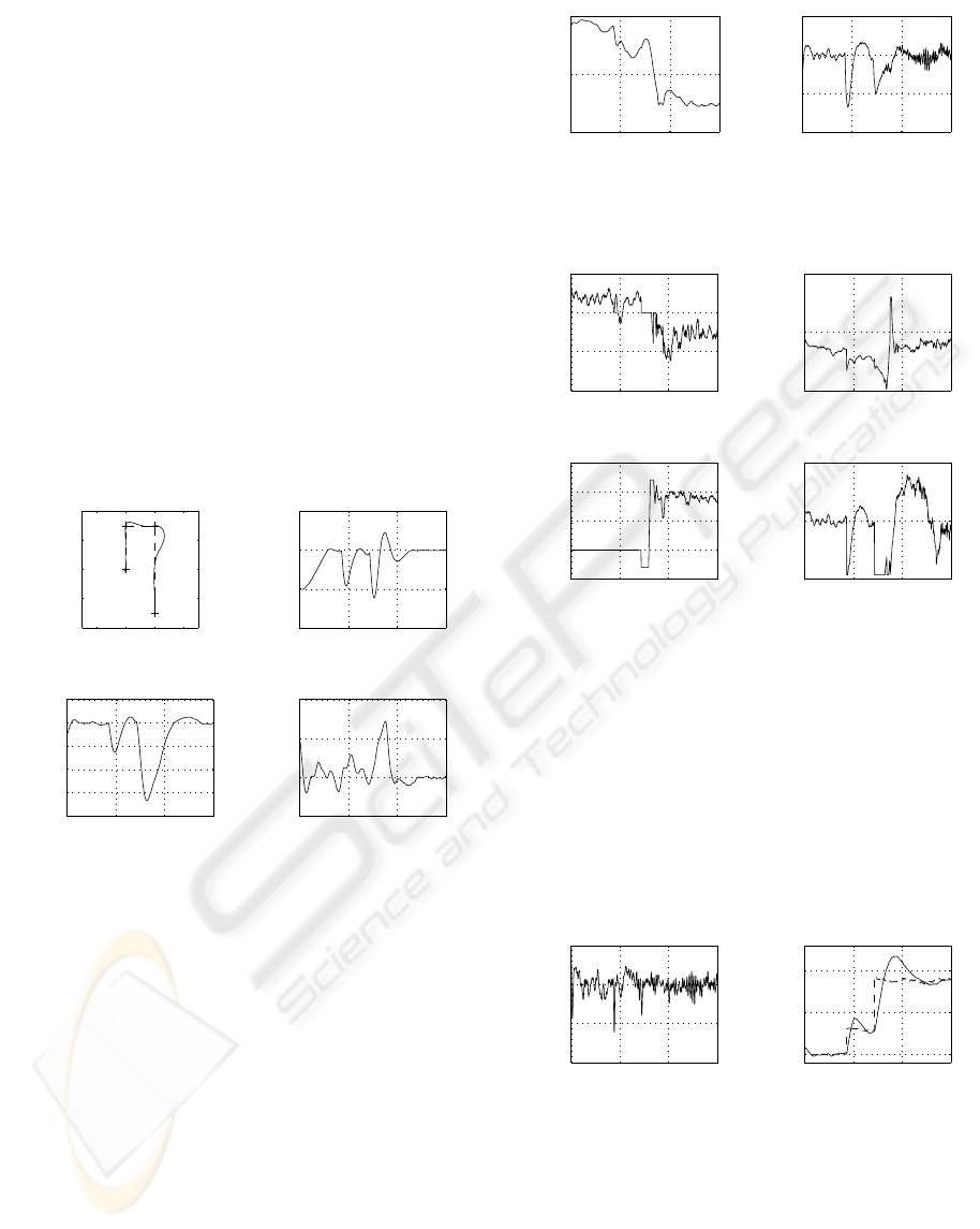
tudinal position error η was limited. This can be no-

ticed by the constant rate at which the north position

is corrected (η curve in ﬁg. 7).

5.2 Realistic Case

In order to exemplify the controller robustness when

in the presence of disturbances, further simulation

tests included a 3D turbulent gust (simulated here by

a Dryden model) with an intensity of 3m/s in addi-

tion to a constant wind blowing at 4m/s from north.

The remaining setup values were the same used in the

previous case.

Figure 8 shows the horizontal north-east trajectory

and the cartesian position errors e

= [η, δ, γ]. The

airship behavior is similar to the nominal case, with

the turbulent gust noticeable by the curves oscillation.

Again, the position errors are corrected to zero, hav-

ing the longitudinal error η been limited to avoid the

thrusters saturation.

East [m]

North [m]

Time [s]

η [m]

Time [s]

δ [m]

Time [s]

γ [deg]

0 50 100

150

50 100 150

0 50 100 150-200

200

400

-5

-80

-60

-40

-20

-40

-20

-400

-200

200

400

Figure 8: Realistic case: north-east trajectory (reference -

dashed, output - solid), and position errors: longitudinal η,

lateral δ and altitude γ.

The evolution of the airspeed V

, represented in ﬁg-

ure 9, deﬁnes the variations of the linear model used

in the control design. The spam of the airspeed val-

ues over the ﬂight envelope, between 2 and 12m/s,

is easily seen. This implies not only that the airship

dynamics suffer a severe alteration, but also the actu-

ators authority varies enormously. This can be con-

ﬁrmed comparing the airspeed curve with the graph-

ics of the actuators input (elevator δ

, total thrust X

vectoring angle δ

and rudder δ

) represented in ﬁg-

ure 10.

Mostly we can observe the vectoring angle δ

change between 0deg for aerodynamic ﬂight, and

90deg at low airspeeds.

The sideslip angle β is also represented in ﬁgure 9.

We can observe that its value oscillates around zero

Time [s]

[m/s]

Time [s]

β [deg]

100

150

50 100 150

-20

-10

Figure 9: Realistic case: airspeed V

and sideslip angle β.

Time [s]

[deg]

Time [s]

[N]

Time [s]

[deg]

Time [s]

[deg]

0 50 100

150

50 100 150

0 50 100 1500

100

150

-25

-50

100

150

100

-20

-10

Figure 10: Realistic case: elevator δ

, total thrust X

, vec-

toring angle δ

and rudder δ

even though the airship is submitted to a wind dis-

turbance. This achievement is due to the fact that the

wind was included in the system model used to obtain

the actuators request.

Finally we can observe in ﬁgure 11 that the rolling

angle φ oscillates around zero, and the variation of the

airship yaw ψ following the reference-path heading.

Time [s]

φ [deg]

Time [s]

ψ [deg]

0 50 100

150

50 100 150

100

200

-20

-10

Figure 11: Realistic case: roll φ and yaw ψ angles (refer-

ence - dashed, output - solid).

As expected for low airspeeds, the control surfaces

authority is reduced, which leads to a slower correc-

tion of the lateral errors in these situations.

A GAIN-SCHEDULING APPROACH FOR AIRSHIP PATH-TRACKING

6 CONCLUSION

In this paper a gain scheduled optimal controller is

designed to solve the path-tracking problem of an air-

ship, valid over the entire ﬂight envelope. The control

law is obtained from a coupled linear model of the

airship that allows to control the longitudinal and lat-

eral motions simultaneously. Due to the importance

of taking into account wind effects, which are rather

important due to the airship large volume, the wind

is included in the kinematics, and the dynamics is ex-

pressed as function of the air velocity.

The examples presented with the inclusion of wind

disturbances, demonstrate the effectiveness of this

single controller tracking a reference path over the en-

tire ﬂight envelope. The implied variation of airspeed

represents a signiﬁcant problem in an airship control

due to its inﬂuence to the system dynamics, as well as

to the actuators authority.

REFERENCES

Astr

om, K. J. and Wittenmark, B. (1989). Adaptive Control,

chapter 9: Gain Scheduling, pages 343–371. Addison-

Wesley Publishing Company, 1

edition.

Azinheira, J. R., de Paiva, E. C., and Bueno, S. S. (2002).

Inﬂuence of wind speed on airship dynamics. Jour-

nal of Guidance, Control, and Dynamics, 25(6):1116–

1124.

de Paiva, E. C., Azinheira, J. R., Ramos, J. J. G., Moutinho,

A., and Bueno, S. S. (2006). Project AURORA air-

ship: Robotic infrastructure and ﬂight control experi-

ments. Journal of Field Robotics.

Elfes, A., Bueno, S. S., Bergerman, M., de Paiva, E. C.,

JR., J. G. R., and Azinheira, J. R. (2003). Robotic

airships for exploration of planetary bodies with an

atmosphere: Autonomy challenges. Autonomous Ro-

bots, (14):147–164.

Elfes, A., Bueno, S. S., Bergerman, M., and Ramos, J. J. G.

(1998). A semi-autonomous robotic airshipfor envi-

ronmental monitoring missions. In Proceedings of the

IEEE International Conference on Robotics and Au-

tomation, volume 4, pages 3449–3455, Leuven, Bel-

gium. IEEE Press.

Hygounenc, E. and Sou

eres, P. (2003). Lateral path-

following GPS-based control of a small-size un-

manned blimp. In Proceedings of the IEEE Interna-

tional Conference on Robotics and Automation, vol-

ume 1, pages 540–545, Taipei, Taiwan. IEEE Press.

Khalil, H. K. (2000a). Nonlinear Systems, chapter 12: Feed-

back Control, pages 485–498. Prentice-Hall, Inc., 3

edition.

Khalil, H. K. (2000b). Nonlinear Systems. Prentice-Hall,

Inc., 3

edition.

Merino, L., Caballero, F., de Dios, J. R. M., and Ollero, A.

(2005). Cooperative ﬁre detection using unmanned

aerial vehicles. In Proceedings of the IEEE In-

ternational Conference on Robotics & Automation,

Barcelona, Spain.

Rao, J., Gong, Z., Luo, J., and Xie, S. (2005). Unmanned

airships for emergency managment. In Proceedings of

the IEEE International Workshop on Safety, Security

and Rescue Robotics, pages 125–130, Kobe, Japan.

IEEE Press.

Rugh, W. J. and Shamma, J. S. (2000). Research on gain

scheduling - survey paper. Automatica, 36(10):1401–

1425.

Silveira, G. F., Azinheira, J. R., Rives, P., and Bueno, S. S.

(2003). Line following visual servoing for aerial ro-

bots combined with complementary sensors. In Pro-

ceedings of the IEEE 11

International Conference

on Advanced Robotics, pages 1160–1165, Coimbra,

Portugal. IEEE Press.

Stevens, B. L. and Lewis, F. L. (1992). Aircraft Control and

Simulation. John Wiley and Sons, Inc., USA.

Xia, G. and Corbett, D. R. (2005). Cooperative control sys-

tems of searching targets using unmanned blimps. In

Proceedings of the 5

Worth Congress on Intelligent

Control and Automation, volume 2, pages 1179–1183,

Hangzhou, P.R.China. IEEE Press.

ICINCO 2006 - ROBOTICS AND AUTOMATION