THE USE OF MODULATING FUNCTIONS FOR
IDENTIFICATION OF CONTINUOUS SYSTEMS WITH
TIME-VARYING PARAMETERS
Witold Byrski, Jedrzej Byrski
Institute of Automatics, AGH University of Science and Technology, Av.Mickiewicza 30, 30059 Krakow, Poland
Keywords: Parameter identification, modulating functions, linear continuous systems.
Abstract: In the paper the use of modulating functions for the optimal identification of the structure and parameters of
continuous linear systems is presented. The modulating functions with compact support [0, h] are used in
convolution filter for transformation of input/output signal derivatives. Based on pre-filtered functions
continuous moving window [t-T, t] is used for on-line identification of piecewise constant parameters Θ
changes of linear system. Optimal quadratic method for identification is presented – with the use of
quadratic constraints on parameters Θ. The numerical results of some examples are shown.
1 INTRODUCTION
One of the continuous model identification method
is based on the use of modulating functions. In 1957
an application of integral transformation with the use
of compact support functions for parameter
identification of differential equation based on input
and output continuous measurement signals given on
[0,T] interval was proposed (Shinbrot, 1957). Such
FIR type filter may be used directly for
identification of continuous systems because of
special properties of convolution.
During primary stage of identification each term
in differential equation is convoluted (multiplying
and integrating) with known modulating functions
on assumed interval [0,T]. Modulating functions and
their derivatives have compact support of length h,
where h<<T, i.e. vanish at the ends of the interval h,
hence initial condition terms of the model also
vanish and finally one can have the new algebraic
(non differential) model with the same unknown
parameters. In the second stage of identification
algorithm, optimal parameter identification problem
is formulated as a problem of minimization of norm
of the equation error in function space L
2
(Byrski
W., 1995, 1996). For nontrivial optimal parameters
solution in optimisation task the constraints for
parameters should be assumed. Assumption of
quadratic constrains of parameters, leads to Gram
matrix G and calculation of their eigenvectors.
Above described methodology one can use for
identification of changes in time-varying parameters,
which are piecewise constant. To this aim the on-
line version of the above method with convolution
filter was prepared and tested. For precise
identification of parameters changes the short
interval T in on-line moving observation window
should be assumed.
Linear time-varying systems were investigated in
many monographs (D’Angelo H., 1970),
Niedzwiecki M., 2000). Publications and references
on identification methods for time-varying
parameters one can find e.g. in survey (Kleiman E.,
2000). However the use of modulating function was
not proposed and tested.
2 MODULATING FUNCTIONS
The idea of using modulating functions and integral
transformation follows from the fact that
convolution of unknown signal derivative y’ and
some known function ϕ is equal to convolution of
original measured signal y and known derivative ϕ’.
Integration by parts shows that the proper choice of
modulating function ϕ with special properties
enables omitting the initial conditions problem
(which are also unknown). Moreover the use of
integral transformation to signals reduces the level
of noise. For identification procedure different
201
Byrski W. and Byrski J. (2006).
THE USE OF MODULATING FUNCTIONS FOR IDENTIFICATION OF CONTINUOUS SYSTEMS WITH TIME-VARYING PARAMETERS.
In Proceedings of the Third International Conference on Informatics in Control, Automation and Robotics, pages 201-204
DOI: 10.5220/0001217802010204
Copyright
c
 SciTePress

modulating function can be chosen. Convolution
filter with different modulation functions has
different filtration properties. The required
properties of modulating functions follow from
below presented identification problem.
Given LTI model of the continuous SISO system
which has to be identified
a
i
y
(i)
(t)
i0
n
b
i
u
(i)
i0
m
(t)=
=
∑
=
∑
(1)
where y
(i)
(t), u
(i)
(t) are the i-th derivatives of the
output and input, respectively, m≤n and the n+m+2
unknown parameters a
i
, b
i
are constant. It can be
assumed that measurements of y and u on the
interval [t
0
,T] are given, where T can be also
considered as the current time.
In order to avoid the difficulties caused by the
presence of derivatives y
(i)
, u
(i)
in the model (1) this
model can be transformed into a more convenient
form by means of convolution. Choosing some
special filtering function ϕ with known derivatives
ϕ
(i)
one can calculate the convolution of the both
sides of model (1) and the function ϕ. This function
ϕ is supposed to be nonzero in interval [0,h] and
zero outside this interval (function with compact
support). The convolution represents continuous
shifting window h along time axis.
[] [][]
==== (t)*y(t)*y(t)*y(t)y
(i)(i)
(i)
df
i
ϕϕϕ
=ττ−ϕτ=
∫
−
)d(t)y(
(i)
t
ht
dτ)(ττ)y(t
(i)
h
0
ϕ
∫
−
(2)
This operation generates the new functions y
i
(t),
u
i
(t), for i=0,..,n(m) for t∈[t
o
+h, T]. Hence the
differential model (1) becomes an algebraic one (3).
Different modulating functions were proposed in
literature (Loeb J., 1965), (Maletinsky V., 1979),
(Preisig H., 1993). In our approach for numerical
tests we will use Loeb-Cahen functions
h][0,t,t)(ht(t)
MN
∈−= ϕ
,
with min(M,N)≥n, N≠M, and n is order of system.
ay(t) bu(t)
ii
i0
n
ii
i0
m
=
==
∑∑
(3)
3 OPTIMAL IDENTIFICATION
For t
0
=0 continuous measurements of the input u and
output y on interval [0,T] are given. We assume that
u, y ∈ L
2
(0,T). After the convolution of both sides of
(1) with an arbitrary assumed function ϕ and with
their derivatives ϕ
(i)
one can obtain new functions
y
i
∈L
2
(h,T), u
i
∈L
2
(h,T) according to (2). The term
ε∈ L
2
(h,T) added to algebraic equation (3) denotes
the combined effects of immeasurable noise or
general equation error EE
a y (t) b u (t) (t)
ii
i0
n
ii
i0
m
=+
==
∑∑
ε
The norm of difference ε(t) of both sides of model
(3) can represent the performance index of
identification.
Denoting by c(t), the vector of convolutions and by
Θ the vector of parameters a
i
, b
i
one can have
[] θε )()(),....,(),(),....,()(
00
tc
b
a
tututytyt
T
mn
=
⎥
⎦
⎤
⎢
⎣
⎡
−−=
The statement of the minimization problem is:
[]
2
L
T
Θ
2
Θ
2
Θ
2
Th,
2
L
(t)Θcminε(t)minJmin ==
Jctct c(tct
TT
L
TT T2
2
===() , () ), ()θθθ θθθG
(4)
The squared norm (4) has a form of inner product in
space L
2
. The real symmetric matrix G is the Gram
matrix of inner products of functions which are
elements of vector c(t)
G =
−−
−−
−−
−−
⎡
⎣
⎢
⎢
⎢
⎢
⎢
⎢
⎤
⎦
⎥
y
0
,y
0
,.., y
0
,y
n
y
0
,u
0
,.., y
0
,u
m
,.., ,.., ,.., ,.., ,.., ,..,
y
n
,y
0
,.., y
n
,y
n
y
n
,u
0
,.., y
n
,u
m
u
0
,y
0
,.., u
0
,y
n
u
0
,u
0
,.., u
0
,u
m
,.., ,.., ,.., ,.., ,.., ,..,
u
m
,y
0
,.., u
m
,y
n
u
m
,u
0
,.., u
m
,u
m
⎥
⎥
⎥
⎥
⎥
,
where inner products are given by formulae
dτds)sτu((s)ds)sτy((s)
τd)(τu)(τyu,y
h
0
(j)
T
h
h
0
(i)
T
h
jiji
⎥
⎦
⎤
⎢
⎣
⎡
−
⎥
⎦
⎤
⎢
⎣
⎡
−
==
∫∫∫
∫
ϕϕ
(5)
ICINCO 2006 - SIGNAL PROCESSING, SYSTEMS MODELING AND CONTROL
202

For avoiding trivial solution Θ = 0 one must chose
the constraints for parameters. The common
constraint used by all researchers is for instance a
n
=1
or a
0
=1 what is interpreted as normalization.
However quadratic constraints are more general.
3.1 Optimal Solution Under
Quadratic Constraints
One can formulate the optimization problem (4) with
unit ball Θ∈B(0,1) constraint for the parameters
}1:{
T22mn
=ΘΘ=Θ∈Θ=
++
RB
(6)
The Lagrangian functional L for the above problem
has a form
)1(GL
TT
ΘΘ−λ+ΘΘ=
From the necessary condition of minimum it follows
directly that
oo
022
L
Θλ=Θ⇒=Θλ−Θ=
Θ∂
∂
GG "
(7)
Hence the optimal element
o
Θ
is an eigenvector of
the Gram matrix G and the Lagrange multiplier λ is
its eigenvalue. From the definition of spectral norm
it follows that the minimum of J
2
on unit ball B(0,1)
is equal to the minimum eigenvalue
[
]
min
T
B
2
B
minJmin λ=ΘΘ= G
(8)
The optimal eigenvector
Θ
o
=w
min
should thus be
chosen, as that which correspond to the minimum
eigenvalue λ
min
of G. Gram matrix G is real and
non-negatively definite. From the formulae (8) one
can find the optimal parameters of (1) and (3) based
on the calculations on interval [0,T]. Such a
parameters represent average value for overall
interval [0,T], (Byrski W., 1999, 2000).
For the current time t>T (in on-line applications)
one should repeated calculations in moving window
[t-T, t]. Then elements of Gram matrix start to be
functions of t and also w(t) and λ
min
(t). Hence
calculations of the minimal λ
min
(t) and eigenvectors
of G(t) should be repeated for every t in interval
[t-T ,t]. The value of Θ(t) represent average value of
parameters for whole interval [t-T ,t]. If the interval
T is short enough it is possible to detect the changes
in system parameters.
4 NUMERICAL TESTS
We present application results of above described
methodology for third order system with time-
varying parameters a
1
, a
2
(piecewise constant
parameters as in Fig.2 and Fig.3 - solid line), b
0
=2.
)()()()()()()(
012
tubtytytatytaty =+
+
+

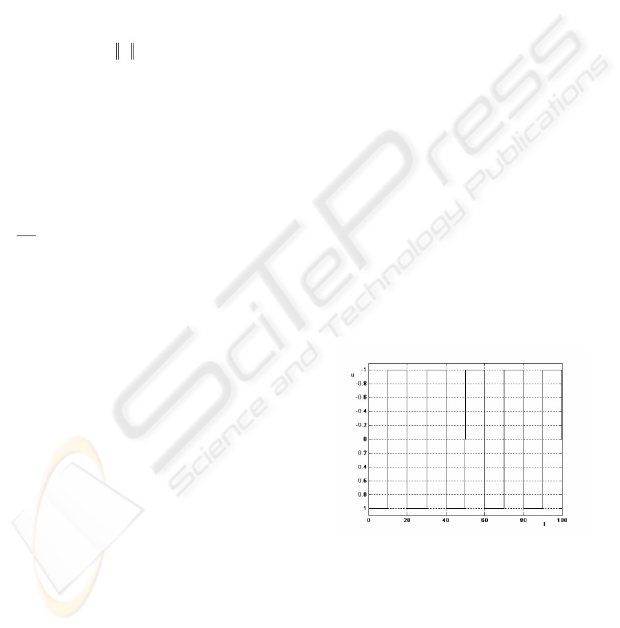
The input and output signals were measured as in
Figure1 and Figure 4. For given input/output vectors
(10000 samples each) program written in C++
automatically searches for the best continuous model
within presumed possibilities.
For starting the program one should prepare the
data file with samples. In this file also, many
possible orders m
i
of input derivative (numerator
degrees of Transfer Function) and many possible
orders n
i
of output derivative (denominator degrees
of TF) should be placed. Also many possible values
of supports h
i
for convolution filter and many
different M, N in ϕ can be proposed. Parameters of
each proper model structure (m
i
≤n
i
) are identified by
the use of different filters based on (2) and (8). Next
each identified model is simulated (by Runge-Kutta
method) and the Output Errors are calculated. The
best model is automatically chosen. Sometimes
different structures give similar small Output Errors
– then special procedure search for the structure,
which is less sensitive to changes of support h
i
in
convoluting filter.
Figure 1: The control signal.
THE USE OF MODULATING FUNCTIONS FOR IDENTIFICATION OF CONTINUOUS SYSTEMS WITH
TIME-VARYING PARAMETERS
203

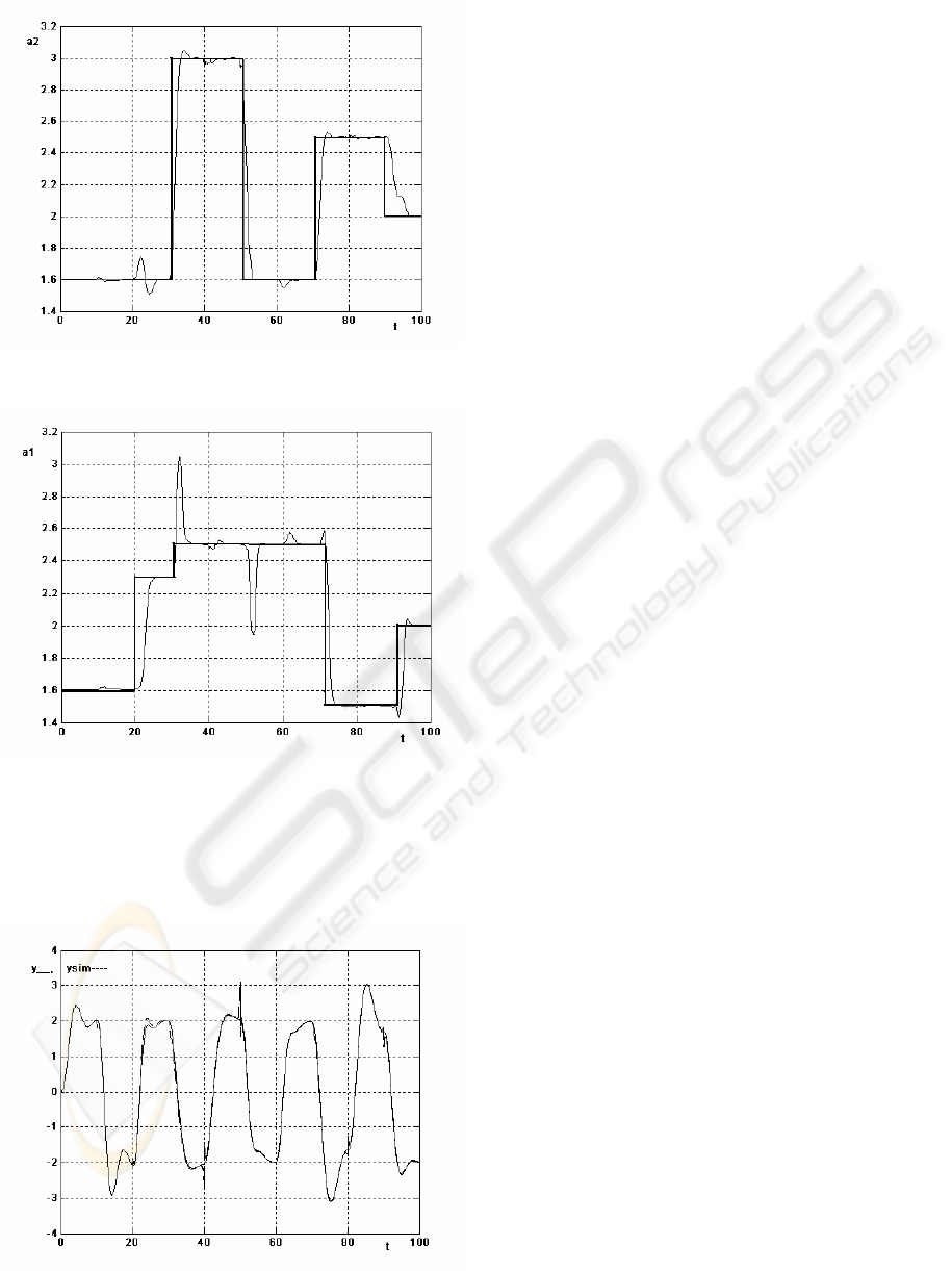
Figure 2: Time-varying parameter a
2
.
Figure 3: Time-varying parameter a
1
.
In Figure 2 and Figure 3 high quality of detection
of rapid parameter changes is observed. Exemplary
result was obtained for T=5, h=1, M=5, N=4. The
differences between measured output and simulated
output presented in Figure 4 are almost invisible.
Figure 4: The outputs of system and model.
5 CONCLUSIONS
In the paper the optimal parameter estimator for
linear continuous systems with time-varying
parameters was presented. The identification method
is based on the convolution of the input/output
measurements with some chosen modulating
function. Preprocessed data are used in Moving
Window Identifier which operates on finite time
interval [t-T ,t], for T<t<T
0
. Hence the solution
gives optimal parameters which are window average
values.
T)(t,
o
Θ
is function of time t and T.
REFERENCES
D’Angelo H., 1970. Linear Time-Varying Systems,
Allyn&Bacon,Boston, USA.
Byrski W., S.Fuksa, 1995. Optimal identification of
continuous systems in L
2
space by the use of compact
support filter. In International Journal of Modelling &
Simulation. IASTED. vol.15 .No.4 .1995. 125-131
Byrski W., S.Fuksa, 1996. Linear adaptive controller for
continuous system with convolution filter. In IFAC,
13th Triennial World Congress, San Francisco USA.
Byrski W., S.Fuksa, 1999. Time variable Gram matrix
eigenproblem and its application to optimal
identification of continuous systems. In Conference
ECC’99, Karlsruhe, Germany.
Byrski W., S.Fuksa, 2000. Optimal identification of
continuous systems and a new fast algorithm for
on-line mode In Proc. of IFAC SYSID2000, Santa
Barbara, USA.
Kleiman E.G., 2000, Identification of Time-varying
Systems-Survey, Proc. of IFAC SYSID2000, Santa
Barbara, USA.
Loeb J, G.Cahen, 1965. More about process identification,
In IEEE Trans.Automat.Control, AC-10.
Maletinsky V.,1979. Identification of continuous
dynamical systems with spline-type modulating
functions method. In Proc. of V IFAC Symp. on
Identification and SPE, Darmstadt, Vol.1.,
Niedźwiecki M., 2000. Identification of Time-varying
Processes, John Wiley, NY.
Preisig H.,A., D.W.T.Rippin, 1993. Theory and
application of the modulating function method.
Review and theory of the method and theory of spline
type modulating functions. In Computers Chem.. Eng.,
Vol.17, No 1,1-40, Pergamon Press.
Shinbrot M., 1957. On the analysis of linear and Nonlinear
Systems. In ASME Trans.. 547-552.
ICINCO 2006 - SIGNAL PROCESSING, SYSTEMS MODELING AND CONTROL
204