BAYESIAN INFERENCE IN A DISTRIBUTED ASSOCIATIVE
NEURAL NETWORK FOR ADAPTIVE SIGNAL PROCESSING
Qianglong Zeng
Bellevue High School,10416 Wolverine Way, Bellevue, WA USA
Ganwen Zeng
Data I/O Corporation, Department of Advanced Technolog,10525 Willows Rd. NE,Redmond, WA USA
Keywords: Bayesian inference, neural network, Adaptive signal processing
Abstract: The primary advantages of high performance associative memory model are its ability to learn fast, store
correctly, retrieve information similar to the human “content addressable” memory and it can approximate a
wide variety of non-linear functions. Based on a distributed associative neural network, a Bayesian
inference probabilistic neural network is designed implementing the learning algorithm and the underlying
basic mathematical idea for the adaptive noise cancellation. Simulation results using speech corrupted with
low signal to noise ratio in telecommunication environment shows great signal enhancement. A system
based on the described method can store words and phrases spoken by the user in a communication channel
and subsequently recognize them when they are pronounced as connected words in a noisy environment.
The method guarantees system robustness in respect to noise, regardless of its origin and level. New words,
pronunciations, and languages can be introduced to the system in an incremental, adaptive mode.
1 INTRODUCTION
Associative neural networks show great potential for
modeling nonlinear systems where it is difficult to
come up with a robust model from classical
techniques. There have been a number of associative
memory structures proposed over the years (Palm
1980; Willshaw and Graham 1995; Palm,
Schwenker et al. 1997), but, as far as the authors
know, there have been no fully functional
commercial products based on best-match
association. In this paper we present what we feel
are the first few steps to creating such a structure in
Bayesian inference. Bayesian inference learning
based associative neural networks can be trained to
implement non-linear functional memory mappings.
This best-match associative network can be viewed
as two outside layers of neurons and multiple inside
hidden layers of neurons, and hence, its operation
can be decomposed into two separate mappings
outside. The input vector is transformed to a vector
of binary values, which in turn produces the sum of
weights that link itself to the corresponding input
vector of value one. As with any training of
perceptron, given an input vector, the desired output
at the output layer can be approximated by
modifying these connection weights through the use
of Bayesian inference learning (Zeng and Dan,
2002). In the output, a match
is defined as a bit for
bit, or exact match (though “don't care” positions
are generally allowed), OR the best match
if there is
no exact match by approximation. Best-match
association then finds the “closest” match according
to some metric distance between the data we
provide and the data in the memory. A number of
metrics are possible. A simple and often used metric
is Hamming distance (number of bits which are
different). However, more complex vector metrics
can be used. A common example of best match
processing is Vector quantization, where the metric
is usually Euclidean distance in a high dimensional
vector space.
There are a number of interesting technical
problems involved in creating a functioning
best-match associative memory system. An
important part of this process that is essential in
many of the potential applications is to be able to
177
Zeng Q. and Zeng G. (2006).
BAYESIAN INFERENCE IN A DISTRIBUTED ASSOCIATIVE NEURAL NETWORK FOR ADAPTIVE SIGNAL PROCESSING.
In Proceedings of the Third International Conference on Informatics in Control, Automation and Robotics, pages 177-181
DOI: 10.5220/0001202101770181
Copyright
c
 SciTePress

formally describe the operation of this memory.
Bayesian Networks and Decision Graphs have been
proposed techniques for modeling intelligent
processes. And there are a number of “intelligent”
applications that are based on Bayesian Networks.
In this paper we propose that Bayesian inference
is an appropriate model for best-match associative
processing. The designed neural network adaptive
learning system is applied to improve the
intelligibility of the speech signal for automatically
adjusting the parameters of the adaptive filter in
order to improve the corrupted speech signal and to
optimize the output signal of the system. The input
signals are stochastic and the information obtained
from the inputs used by the adaptive algorithm is to
adjust the weights and to achieve parameter
adjustments close to optimum. Most of the
conventional work towards canceling noise to
improve the corrupted speech signal uses the Least
Mean Squared (LMS) algorithm, or Recursive Least
Square (RLS) algorithm to cancel of the unwanted
noise under the assumption that a reasonably good
model of the actual unwanted signal is available.
The noise estimate, or sometimes referred to, as the
reference signal, could not be correlated to the
speech signal to be recovered, as this will cancel the
actual speech as well.
The simulation results show an increased
performance of the Bayesian Networks compared to
the conventional RLS adaptive algorithm.
2 NEURAL NETWORK FOR
NOISE CANCELLATION
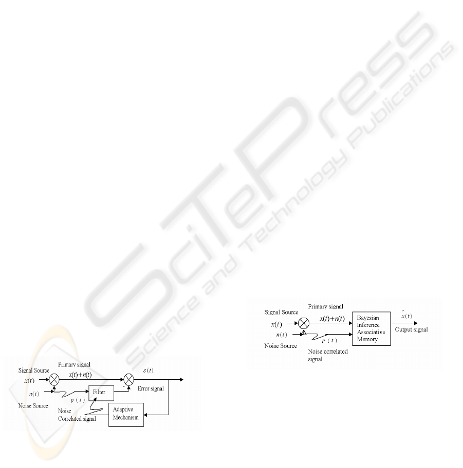
Figure 1 shows a conventional adaptive noise
cancellation scheme where
)(tx
represents a
noiseless signal and
)(tn
a superimposed noise.
Figure 1: LMS/RLS Based Adaptive Noise Cancellation.
An adaptive filter in the feedback loop tailors a
noise-correlated input
)(tp
and outputs the estimate
)(tm
of the noise
)(tn
. The error function is then
given by
)()()()( tmtntxt −+=
ε
With a mean-square deviation
))()()((2))()(()()(
222
tmtntxtmtntxt −+−+= ε
That yields the expectation function
))
]
()()((2[]))()([()]([)]([
222
tmtntxEtmtnEtxEtE −+−+= ε
If
)()( tntx
⊥
,
)()( tmtx
⊥
, one has
]))()([()]([)]([
222
tmtnEtxEtE −+= ε
Since
)]([
2
txE
isn’t affected by the adaptive
mechanism itself,
]))()([(
2
tmtnE −
can be
minimized for a given
)(tp
by the Least Mean
Squared (LMS) algorithm, or Recursive Least
Square (RLS) algorithm; i.e.,
0]))()([(
2
≈− tmtnE
so we will have
)]([)]([
22
txEtE ≈ ε
, then
)()( txt ≈
ε
.
The proposed neural network noise cancellation
is a Bayesian inference based distributed associative
neural network (shown in Figure 2 where the
output
)()(
^
txty =
,
)(
^
tx
is the signal estimate). It
constructs a Bayesian inference associative memory
(BIAM) neural network to suppress noise and to
output the signal estimate. The BIAM neural
network consists of multiple clusters of
self-organizing feature maps. The weights in the
BIAM neural network are effectively the
coordinates of the locations of the neurons in the
map. The output of the winning neuron can be
directly obtained from the weight of a particular
output neuron. Instead of storing the signal estimate,
BIAM memory only stores the weight, which
represents the functions of the outputs of the
estimate signal and the estimate noise spectra in the
association engine.
Figure 2: BIAM Neural Network Noise Suppression.
3 PALM ASSOCIATION
For the first association engine, we want an
algorithm that is reasonably well understood and
performs robust best-match association
computation. Figure 3 shows the architecture of
BIAM for noise cancellation.
In Figure 3, TDL is a tapped delay line. The
input signal such as the primary
ICINCO 2006 - SIGNAL PROCESSING, SYSTEMS MODELING AND CONTROL
178

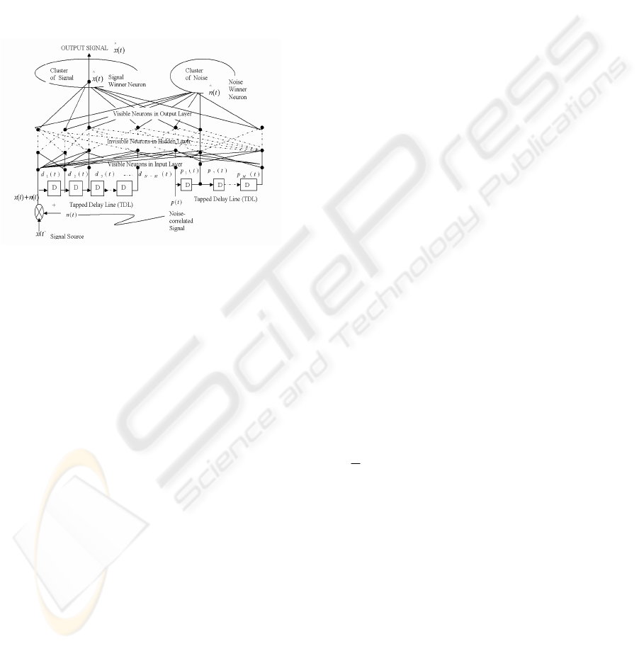
signal
)()( tntx +
and the noise-correlated input
)(tp
enters into a TDL, and passes through N-1
delays for the primary signal and M-1 delays for the
noise-correlated input. The output of the tapped
delay line (TDL) is an (N+M)-dimensional vector,
made up of the input signal at the current time, the
previous input signal, etc. MIAM competitive
learning will output the signal winner neuron
through the weights of the cluster of neurons. It
separates the noise winner neuron in the noise
cluster. The learning only occurs in the output
neurons.
Figure 3: Architecture of BIAM for Noise Cancellation.
As a first pass, we have chosen to use the simple
associative networks of Günther Palm (Palm, 1997
#82). Part of the purpose of using Palm is as a driver
for the design methodology. We have no intention
of limiting ourselves to that model and feel that
many more interesting and powerful models will be
available for us.
The algorithm stores mappings of specific input
representations
i
x
to specific output
representations
i
y
, such that
ii
x
y→ . The network
is constructed via the input-output training
set
(, )
ii
x
y , where ()
ii
Fx y
=
. The mapping F is
approximative or interpolative in the sense that
()
ii
Fx y
ε
δ +=+, where
i
x
ε
+ is an input
pattern that is close to input
x
μ
being stored in the
network, and
ii
xy =
with
0))()((
^
→−= tntn ε
and
0→
δ
. This definition also requires that a
metric exists over both the input and output spaces.
We are using a simplified auto-association
version of Palm’s generic model, where the input
and output are the same. Furthermore, all vectors
and weights are binary valued (0 or 1) and have
dimension N. There is also a binary valued n by n
matrix that contains the weights. Output
computation is a two step process. First an
intermediate sum is computed for each node (there
are also n nodes).
[, ]'[]
N
j
k
s
wjkxk=
∑
In the notation, a vector x’ is input, an inner
product is computed between the elements, k, of the
input vector and each row, j, of the weight matrix.
For auto-association the weight matrix is square and
symmetric.
The node outputs then are computed
ˆ
()
j
jj
xfs
θ
=
−
The function, f, is a non-linear function such as a
sigmoid. We are currently assuming a simple
threshold function whose output
ˆ
j
x
then is 1 or 0
depending on the value of the node’s threshold
j
θ
.
The setting of the threshold is complex and will be
discussed in more detail below. Initially we shall
assume that there is one global threshold, but we
will relax that requirement as we move to modular,
localized network structures.
The next important aspect of these networks is
that they are “trained” on a number of training
vectors. In the case of auto-association, these
represent the association targets. In the Hopfield
energy spin model case, these are energy minima.
There are M training or memory patterns. In the
auto-associative memories discussed here the output
is fed back to the input so that X=Y.
The weights are set according to a “Hebbian”
like rule. That is, a weight matrix is computed by
taking the outer product of each training vector with
itself, and then doing a bit-wise OR of each training
vector’s Hebbian matrix.
1
()
M
ij i j
wxy
μ
μ
μ
=
=
∪
The final important characteristic is that only a
fixed number of nodes are active for any vector. The
number of active nodes is set so that it is a relatively
small number compared to the dimensions of the
vector itself – Palm suggests
(log( ))aO N= . It is
worth noting that the LMS algorithm operates in
O(N) operations per iteration, where N is the
number of tap weights in the filter, whereas RLS
uses O(N^2) operations per iteration. Although
reducing theoretical capacity somewhat, small
values of a lead to very sparsely activated networks
and connectivity. It also creates a more effective
computing structure. Training vectors are generated
with only nodes active (though in random
BAYESIAN INFERENCE IN A DISTRIBUTED ASSOCIATIVE NEURAL NETWORK FOR ADAPTIVE SIGNAL
PROCESSING
179

positions). Likewise, we have assumed that test
vectors, which are randomly perturbed versions of
training vectors, are passed through a saturation
filter that activates only a node. This is also true of
network output, where the global threshold value
(which is the same for all nodes),
θ
, is adjusted to
ensure that only the K nodes with the largest sums
are above threshold— this is known as K
winners-take-all (K-WTA). Palm has shown that in
order to have maximum memory capacity, the
number of 1s and 0s in the weight matrix should be
balanced, that is p
1
= p
0
= 0.5, that is
0
ln ln 2Mpq p=− ≤ . In order for this relationship to
hold, the training vectors need to be sparsely coded
with log n bits set to 1, then the optimal capacity
69.02ln =
is reached.
3.1 Palm Association as Bayesian
Inference
Message x
i
is transmitted, message
)()()(
'
tntxtx +=
is received, and all vectors are
N bits in length, so the Noisy Channel only creates
substitution errors. The Hamming Distance between
these two bit vectors is HD(x
i
, x
j
). We are assuming
throughout the rest of this paper that the Noisy
Channel is binary symmetric with the probability of
a single bit error being ε, and the probability that a
bit is transmitted intact is (1-ε). The error
probabilities are independent and identically
distributed and ε < 0.5.
We can now prove the following result:
Theorem 1: The messages, x
i
, are transmitted
over a Binary Symmetric Channel and message x’ is
received. For all messages, x
i
, being equally likely,
the training vector with the smallest Hamming
Distance from the received vector is the most-likely
that was sent in a Bayesian sense,
,min (,')
ii
ist HDx x∀ and
,max(|')
ij
jst px x∀ , i=j
Proof: This is a straightforward derivation from
Bayes rule
1
['| ][ ]
[|']
['| ][ ]
ii
i
N
j
j
j
px x px
px x
px x px
=
=
∑
Since the denominator is equal for all inputs, it
can be ignored. And since the x
i
are all equally
likely the p[x
i
] in the numerator can be ignored. Let
x
i
(h) be a vector that has a single bit error from x
i
,
that is HD(x
i
(h), x
i
)=h. The probability, p(x(1)) of a
single error is (1-ε)
n-1
ε. Note, this is not the
probability of all possible 1-bit errors only the
probability of a single error occurring that
transforms x
i
into x’. The probability of h errors
occurring is, p(x(h)) = (1-ε)
n-h
ε
h
. It is easy to see that
for ε<0.5 then p(x(1)) > p(x(2)) > … > p(x(h)). And
by definition HD(x(1)) < HD(x(2)) < … <
HD(x(h)). By choosing the training vector with the
smallest Hamming Distance from x’, we maximize
['| ]
i
p
xx and thus maximize [|']
i
p
xx
Theorem 2: When presented with a vector x’,
the Palm association memory returns the training
vector with the smallest Hamming Distance, if the
memory output is that vector x
i
, then we have
min ( , ')
ii
HD x x
The proof is not given here, but this is a
fundamental property of the Palm network as shown
by Palm (Palm 1980).
Going back to Bayes’s rule, using the fact that
the probability of h errors is p(x(h)) = (1-ε)
n-h
ε
h
, and
taking the logarithm we get:
ln [ ( | ')] ln [(1 ) ] ln[ ( )]
( , ')(ln ln (1 )) ln ( )
Nh h
i i
ii
px x px
HD x x p x
εε
εε
−
=− +
=−−+
Setting
(ln ln(1 ))
α
εε
=
−−and dividing, we
get
( , ') ( , ') ( )
iii
f
xx HDxx fx
=
+
Where f is the log of the probability, divided by
α.
We can then create a modified Palm network
‘with priors’ where there is a new input for each
vector. This input adds to the accumulating inner
product.
The weights in this modified Palm network are
calculated according to a “Hebbian” like rule and
the knowledge of prior probabilities. That is, a
weight matrix is computed by taking the outer
product of each training vector with itself, and then
doing a bit-wise OR of each training vector’s
Hebbian matrix; and plus an inference-based
learning item. η is a learning rate.
Theorem 3: The message x
i
is transmitted over a
Binary Symmetric Channel and message x’ is
received. For all messages, x
i
, with probability of
occurrence p(x
i
), the training vector with the
smallest Weighted Hamming Distance from the
received vector, x’, is the most likely message sent
in a Bayesian sense,
,max(,')
ii
ist f x x
∀
and
,max(|')
ij
ist px x
∀
, i=j.
Proof: The proof is similar to Theorem 1
ICINCO 2006 - SIGNAL PROCESSING, SYSTEMS MODELING AND CONTROL
180

Based on the given prior probabilities of the
training messages, the weights are learned by
inference of the closest stored pattern. It minimizes
the objective function HD(x
i
, x’); this gives to
This means the Palm reference associative
memory can most likely recall the store x
i
from
noised message input x’. It makes the message x
i
be
recalled independently to its noise signal.
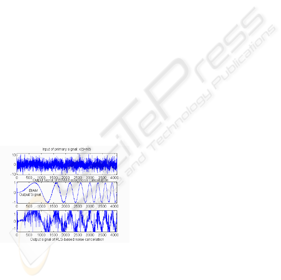
4 CONCLUSION
In our implementation of the BIAM algorithm for
noise cancellation we modeled the additive noise as
a random white Gaussian process. We model the
unknown acoustical system as a randomly generated
FIR filter. We used sine chirps and a voice
recording for our input signals. The simulation in
Figure 4 observed with our experiments, BIAM has
significantly faster convergence behavior than the
conventional LMS/RLS. In general, it seems to
converge within log (N) iterations, where N is the
number of tap weights having a better steady state
approximation of tap weights. This significantly
improves the final noise removal performance.
These results demonstrate that the Palm memory is
operating as a Bayesian classifier.
Figure 4: Simulation Result.
REFERENCES
Zeng, G., and Dan, H., Distributed Associative Neural
Network Model Approximates Bayesian Inference,
Proceedings of the Artificial Neural Networks in
Engineering Conference (ANNIE 2002), pages 97-103,
St. Louis, Missouri, Nov 2002.
Jensen, F., The book Bayesian Networks and Decision
Diagrams, Springer. 2001.
valueaxfxxf
ii
min)(),(
'
⇒−
BAYESIAN INFERENCE IN A DISTRIBUTED ASSOCIATIVE NEURAL NETWORK FOR ADAPTIVE SIGNAL
PROCESSING
181