
KEY PERFORMANCE INDICATORS IN PLANT-WIDE
CONTROL
Sebastjan Zorzut, Vladimir Jovan
Jozef Stefan Institute, Jamova 39, SI-1000 Ljubljana, Slovenia
Alenka Žnidaršič
Metronik d.o.o., Stegne 9a, SI-1000 Ljubljana, Slovenia
Keywords: Key performance indicators; Production management; Decision support systems; Closed-loop control.
Abstract: To improve production performance it is necessary to define production goals with a proper implementation
strategy and a suitable closed-loop control for their achievement. A promising solution is the use of the Key
Performance Indicators (KPIs) approach. To verify the idea of production feedback control using production
KPIs as referenced controlled variables, a procedural model of a production process for a polymerisation
plant has been developed. The model has been used during a number of simulation runs performed with the
aim of developing and verifying the idea of KPI-based production control.
1 INTRODUCTION
A production process involves several business and
technical activities on and around the factory floor.
Its effectiveness can be assessed using information
hidden in a set of current and historical production
data. The problem of extracting the relevant
information from production data for fast and
accurate decision-making can be solved by
introducing a set of production KPIs (Vicens et al,
2001; Lohman, 2003) that show the operational and
mid-term efficiency of the production. On the
strategic management level, the problem of overall
business efficiency in a production factory is already
being solved with this approach (DeBusk, 2003),
while on a production management level the
implementation of KPIs is a rather new concept. The
solution lies in defining an appropriate set of KPIs
that are specific to the observed production process,
and in defining the strategy for using KPIs to
efficiently manage that process. Recently, a
balanced set of general KPIs for the production
management level has already been introduced
(Rakar et al, 2004) and five principal KPIs for
process-oriented productions were defined: Safety
and Environment; Production Efficiency; Production
Quality; Production Plan Tracking; and Employees
Issues.
2 CLOSED-LOOP PRODUCTION
MANAGEMENT PARADIGM
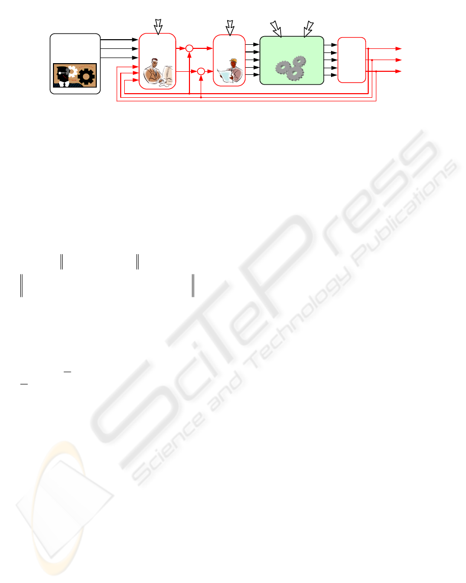
The desired global production objectives in the
context of production management system can be
more objectively defined as the reference values for
significant measures of plant efficiency, production
plant productivity, mean product quality and others.
These production objectives are often called implicit
objectives as they usually can be expressed only
implicitly as functions of the measurable and
manipulatable variables (Stephanopoulos and Ng,
2000). Since implicit objectives are not directly
measurable, their translation into a set of output
production process variables should be provided.
These output production process variables should
have the following properties (Skogestad, 2004): (i)
they should be more easily measurable, (ii) it must
be possible to handle maintaining their set point
values by proper adjustments of manipulatable
production process variables, and (iii) when
maintained at the desired optimal set-points through
the feedback control subsystem, they should
inherently contribute to the overall profitability of a
production process. These variables are denoted in
this paper as “production KPIs” (see Figure 1).
179
Zorzut S., Žnidarši
ˇ
c A. and Jovan V. (2006).
KEY PERFORMANCE INDICATORS IN PLANT-WIDE CONTROL.
In Proceedings of the Third International Conference on Informatics in Control, Automation and Robotics, pages 179-182
DOI: 10.5220/0001201301790182
Copyright
c
SciTePress
This production control problem can be
mathematically formulated as in (Stephanopoulos
and Ng, 2000):
Let z
PROFIT
represents the operating profit:
. costs production
costs materialraw luesproduct vaz
PROFIT
∑
∑∑
−
−−=
The feedback-based solution leads to the
following optimisation problem:
),,(z),,(zmin
zzMinimize
PROFITPROFIT
C(.)sp,,y,u
PROFITspPROFIT,
fbfb
dyudyu −
=−
subject to
).(
u
esdisturbanc process
sconstraint process 0 ) , ,(
dynamicsplant ) , ,(
fbfb
fb
yCu
UU
Dd
dyug
dyuhy
=
≤≤
∈
≤
=
where, u
fb
and y
fb
denote the manipulations and
measurements involved in the feedback-based
solution and C is the structure of the entire
production control system.
3 THE CASE STUDY
The polymer emulsion batch production process
taken in this paper for the case study is a typical
representative of process-oriented production where
production effectiveness to a great extent relies on
the quality of the production control system. The
process is described in more details in (Jovan and
Zorzut, 2006).
A procedural model of the case study
production process has been developed to facilitate
experimenting and the verification of the closed-
loop control structure. The model was designed in
the academically established Matlab, Simulink and
Stateflow simulation environments. The simulated
data are stored in the MS Access database and are
available for different on-line or off-line processing.
Given the final objective of stabilising the
existing production process, a promising idea is to
introduce a closed-loop production management
concept so that specific production KPIs serve as the
reference values for the closed loop production
control system. It is hypothesised that such an
approach can contribute to more stable production
and better final product uniformity and quality.
Three production KPIs were chosen to characterise
the case study production process:
• Productivity (also denoted as actual production
rate or production yield). Productivity is defined for
the described production process as the amount of
all products that were produced over a set
production period. All batches finished within the
set time window (production period) are taken into
account and the average amount of products
produced in an hour is calculated.
• Mean Product Quality. The Mean Quality KPI is
calculated as the mean value of the quality factors
for the batches completed in the set time window.
• Mean Production Costs. Production costs consist
of raw material costs, energy costs, other operating
costs and fixed costs in the set time window. The
mean production costs are calculated as the sum of
all production costs within a time window, divided
by the amount of all products produced in this time
window.
These three KPIs represent the output
(controlled) variables on Figure 1. Maintaining the
predefined set points for these KPIs is achieved by
properly adjusting the manipulated (input) variables,
which are in this case: Raw Material Quality,
Production Speed and Batch Schedule. Determining
the influence of the input variables and disturbances
on the output variables (selected KPIs) is essential
for efficient production control.
PRODUCTION
PROCESSES
Energy and
raw materials
Disturbances
WHAT
HOW MUCH
WHEN
Productivity
Quality
Costs
+
-
+
-
MANAGEMENT
LEVEL
Technological
constraints
Economic
issues
Production
manager
using DSS
Operator
using
DSS
Key
Performance
Indicators
Figure 1: Closed-Loop Control Structure of the Production Process.
ICINCO 2006 - INTELLIGENT CONTROL SYSTEMS AND OPTIMIZATION
180
3.1 Simulation Runs
To see how the production speed and the quality of
raw materials affect productivity, product quality
and production costs, a simulation run was
performed. Simulation run was divided in three
phases, where the production speed was changed
from low to normal and finally to high. On Figure 2
the first phase lasts from 0 to 450 hours of
simulation time, the second phase from 450 to 870
hours and the third phase from 870 till the end. In
each phase the quality of the raw materials was
subsequently increased from low to very high (0.85
to 1.1). The KPIs for Product Quality, Productivity
and Production Costs were observed. The KPIs were
evaluated every 12 hours for the time window of 120
hours.
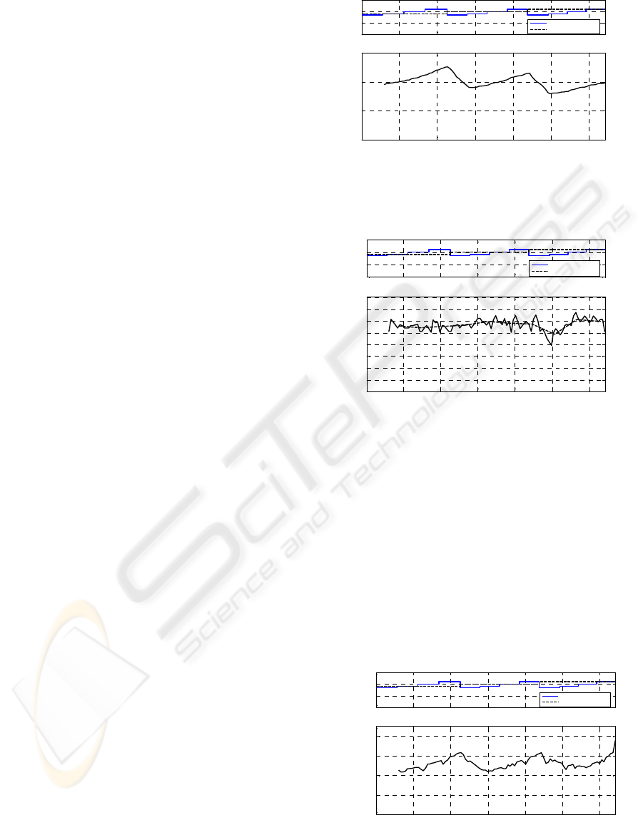
Figure 2 represents the response of the Product
Quality KPI. In the first phase of the simulation run
the production speed was low, which represents the
best working conditions in the production process.
Over the simulation run the quality of raw materials
gradually increased and the influence of this change
on the Product Quality KPI can be observed. As
expected, better quality raw materials contribute to
better quality final products.
In the second phase of the simulation run the
production speed is increased, which usually leads to
decreasing production process quality. Raw material
quality changed in the same manner as in the
previous phase: from low to high. The Product
Quality KPI first decreased and when it reached the
bottom it started increasing as in the first phase. The
change in product quality is momentary but the
change in the Product Quality KPI is gradual. The
KPI evaluation algorithm averages the product
quality in the set time window, which can be seen in
this section of the figure. The second interesting
phenomenon is the influence of production process
quality on product quality. The mean quality of the
products decreases by about 10 %. In the third phase
the pattern is repeated.
Figure 3 represents the Productivity KPI for the
same simulation run. The Productivity KPI has
slightly increasing trend with higher production
speed. At the beginning of the third phase of the
simulation run high production speed causes the
significant decrease of productivity. This is the
result of coincidence that the quality of the
production process and also the quality of the raw
materials are low. Consequently, some batches do
not attain prescribed quality requirements and they
have to be recycled, what affects Productivity KPI.
The appearance of off-spec batches can be noticed
0 200 400 600 800 1000 1200
0
0.5
1
1.5
Raw materials quality and production rate
Raw materials quality
Production rate
0 200 400 600 800 1000 1200
0
0.5
1
1.5
Mean product quality for the time window: 120h
Prod uc tion time(h)
Mean product quality
Figure 2: Response of the Mean Product Quality KPI to
Raw Material Quality and Production Speed.
0 200 400 600 800 1000 1200
0
0.5
1
1.5
Raw materials quality and production speed
Raw materials quality
Production speed
0 200 400 600 800 1000 1200
0
200
400
600
800
1000
1200
1400
1600
Produc tiv ity for the time window: 120h
Production time(h)
P
ro
d
uc
ti
v
it
y
(k
g
/h)
Figure 3: Response of the Productivity KPI to Raw
Material Quality and Production Speed.
on the Figure 3 (time period from 900 to 950 hours)
where the reactor occupancy for some batches is
increased due to the need of recycling of bad batches
entering in the production process.
Figure 4 represents the mean Production Costs
KPI. The production costs per product unit increase
with the increasing quality of raw materials. There is
a slight increase in costs with increasing production
speed.
The following simulation run presents the open-
loop control of the Product Quality KPI.
0 200 400 600 800 1000 1200
0
0.5
1
1.5
Raw materials quality and production rate
Raw materia ls quality
Production rate
0 200 400 600 800 1000 1200
0
50
100
150
200
Mean product cost for the time window: 120h
Production time(h)
M
ean pro
d
uc
t
cos
t
(Sit/k
g
)
Figure 4: Response of the Mean Production Costs KPI to
Raw Material Quality and Production Speed
.
KEY PERFORMANCE INDICATORS IN PLANT-WIDE CONTROL
181

0 50 100 150 200 250 300 350 400
0
0.5
1
1.5
Raw materials quality and production speed
Raw materia ls quality
Production speed
0 50 100 150 200 250 300 350 400
0
0.2
0.4
0.6
0.8
1
1.2
Mean product quality for the time window: 75h
Production time (h)
Mean product quality
Figure 5: Open-Loop Control of the Product Quality KPI.
The experiment represents the execution of a normal
schedule of production jobs using raw materials with
normal quality at normal production speed. After a
certain time period, a disturbance occurs in the form
of a decrease in the quality of raw materials, which
is reflected in the considerable decreased value of
the mean of the Product Quality KPI (see Figure 5).
As an open-loop control action the production
manager then slows down current production speed.
The quality of both the production process and final
product gradually increase, and consequently this is
reflected in the increase in the mean value of the
Product Quality KPI. This is not the only possible
action that production manager could take, but in the
presented case it was sufficient to eliminate the
disturbance.
4 CONCLUSIONS
The ideal plant-wide control system should ensure
that the production process is constantly working in
an optimal manner. As a result of the plant-wide
focus, a plant-wide control problem possesses
certain characteristics that are not encountered in the
design of control systems for single units, such as
the following (Stephanopoulos and Ng, 2000): (a)
the variables to be controlled by a plant-wide control
system are not as clearly or as easily defined as for
single units; (b) local control decisions, made within
the context of single units, may have long-range
effects throughout the plant; (c) the size of the plant-
wide control problem is significantly larger than that
for the individual units, making its solution
considerably more difficult.
This paper proposes an approach to measuring
and presenting the attainment of production
objectives in the form of production KPIs. With this
approach the implicit production objectives were
translated into measurable values that can be
extracted from existing production data. In this way
the production control concept and the role of a
production manager are slightly changed; instead of
monitoring and controlling several tens and
hundreds of process variables at a low production
level, a production manager monitors and controls
only a few major production KPIs with the aim of
achieving the most important implicit production
objectives, e.g. high product quality, high
productivity and minimal production costs.
The procedural model of the case study
production process has been developed and used in a
number of simulation runs. The preliminary
simulation results presented indicate that this work
could evolve towards the implementation of a
production KPI-based control system in a real
industrial plant. The intention in future is to improve
the existing production process model, validate it
rigorously and incorporate it into a Decision Support
System for production control in the polymerisation
plant that was used as the case study production
process in this paper.
REFERENCES
DeBusk, G. K., Brown, R. M., Killough, L. N. (2003):
Components and relative weights in utilization of
dashboard measurement systems like the Balanced
Scorecard, The British Accounting Review, Volume
35, Issue 3, pp. 215-231.
Jovan, V. and Zorzut, S. (2006): Use of Key Performance
Indicators in Production Management, Proceedings of
the IEEE International Conference on Cybernetics
and Intelligent Systems, 7.-9. June, Bangkok, 2006.
Lohman, C., Fortuin, L., Wouters, M. (2004): Designing a
performance measurement system: A case study,
European Journal of Operational Research 156,
Elsevier press, pp. 267-286.
Rakar, A., Zorzut, S., Jovan, V. (2004): Assesment of
production performance by means of KPI,
Proceedings of the Control 2004, 6-9 September,
2004, University of Bath, UK.
Skogestad S. (2004): Control structure design for complete
chemical plants, Computers and Chemical
Engineering 28, pp. 219-234.
Stephanopoulos G., Ng C. (2000): Perspectives on the
synthesis of plant-wide control structures, Journal of
Process Control 10 (2000), pp 97-111.
Vicens, E., Alemany M. E., Andres C., Guarch J. J.
(2001): A design and application methodology for
hierarchical production planning decision support
system in an enterprise integration context, Int.
Journal of Production Economics 74, Elsevier Press,
pp. 5-20.
ICINCO 2006 - INTELLIGENT CONTROL SYSTEMS AND OPTIMIZATION
182
