Using Restricted Random Walks for Library

Recommendations

Markus Franke and Andreas Geyer-Schulz

Institut f

ur Informationswirtschaft und -management

Universit

at Karlsruhe (TH), 76128 Karlsruhe, Germany

Abstract. Recommendations are a valuable help for library users e.g. striving

to gain an overview of the important literature for a certain topic. We describe

a new method for generating recommendations for documents based on cluster-

ing purchase histories. The algorithm presented here is called restricted random

walk (RRW) clustering and has proven to cope efﬁciently with large data sets.

Furthermore, as will be shown, the clusters are very well suited for giving recom-

mendations in the context of library usage data.

1 Motivation and Introduction

Services like amazon.com’s “Customers who bought this book also bought . . .” are an

important service – for all involved parties: The customer receives assistance in ﬁnding

his way through the range of books offered by the shop, the bookseller has the possibil-

ity to increase its sales by proposing complementary literature to its customers [1].

Technically, a recommender service can be implemented in different ways. We will

present an innovative approach based on a fast clustering algorithm for large object

sets [2] and making use of product cross-occurrences in purchase histories: In our case,

the purchase histories are those of users of the Online Public Access Catalogue (OPAC)

of the university’s library at Karlsruhe, and a purchase is the viewing of a document’s

detail page in the WWW interface of the OPAC. A cross-occurrence between two doc-

uments is given when their detail pages have been viewed together in one user session.

Following the standard assumption for behavior-based recommender systems, we

assume that a high number of cross-occurrences hints at a high complementarity of two

documents that we can interpret in the recommender context as similarity.

The paper is structured as follows: We start by outlining existing recommender

systems and cluster algorithms in section 2. In section 3 we will present the restricted

random walk clustering algorithm before discussing the generation of recommendations

from clusters in section 4. Results will be shown in section 5 and a conclusion as well

as an outlook onto further research topics are given in section 6.

2 Recommender systems and Cluster Algorithms for Library

OPACs

General classiﬁcation schemes for recommender systems have been presented by Resnick

and Varian [3], by Schafer et al. [1], and Gaul et al. [4].

Franke M. and Geyer-Schulz A. (2005).

Using Restricted Random Walks for Library Recommendations.

In Proceedings of the 1st International Workshop on Web Personalisation, Recommender Systems and Intelligent User Interfaces, pages 107-115

DOI: 10.5220/0001412001070115

 SciTePress

The systems we will scrutinize more closely are so-called implicit recommender

systems that generate recommendations from user protocol data – e.g. purchase his-

tories at the (online) store, Usenet postings or bookmarks – without the need of user

cooperation. This distinction between implicit and explicit recommender systems is

important since no additional customer effort is necessary to gain these recommenda-

tions and thus incentive-related problems like free riding or bias are minimal. This has

been discussed e.g. by Geyer-Schulz et al. [5] or Nichols [6].

All recommender systems mentioned here have in common that they do not perform

content analysis, contrary to information retrieval based methods as described for in-

stance by Semeraro [7], Yang [8] and others. This is important since in a hybrid library

like the one in Karlsruhe, only a fraction of the corpus is available in digital form.

Currently, two methods are being broadly used to generate recommendations from

purchase histories: A straightforward one employed for instance by amazon.com, and

an LSD model based approach using Ehrenberg’s repeat buying theory [9] used for

example at the university library in Karlsruhe [10].

The ﬁrst approach is to recommend the books that have been bought (or viewed)

most often together with the book the customer is currently considering. The challenges

of this idea lie mainly in its implementation for large data sets, even if the matrix of

common purchases is quite sparse.

Another, more sophisticated model makes use of Ehrenberg’s repeat buying the-

ory [9, 10]. Its advantage lies in a noticeably better quality of the recommendations,

because the underlying assumption of a logarithmic series distribution allows to distin-

guish between random and meaningful cross-occurrences in a more robust way.

However, these recommender systems only take into account direct neighborhoods

in the similarity graph generated by the purchase histories. Each extension that includes

the neighbors of the neighbors into the recommendations quickly becomes computa-

tionally intractable. This is not the case with cluster-based recommender systems: the

recommendations do not only contain the documents directly related to each other, but

the clusters also account for indirect relations where this is necessary.

For a general overview of clustering and classiﬁcation algorithms, we refer to Duda

et al. [11] or Bock [12]. In the past there have been some proposals for recommender

systems or collaborative ﬁltering based on cluster algorithms [13,14].

We chose restricted random walk clustering for two reasons: Its ability to cope with

large data sets that will be discussed in section 3.4 and the quality of its clusters with

respect to library purchase histories.

Viegener [15] investigated the use of cluster algorithms for the construction of a

library’s thesaurus extensively. On the one hand, Viegener’s results are encouraging be-

cause he found semantically meaningful patterns in library data. On the other hand,

all standard cluster algorithms proved to be computationally expensive – Viegener’s

results were computed on a supercomputer at the Universit

at Karlsruhe that is not avail-

able for routine library operations. Besides, the quality of the clusters generated by the

algorithms scrutinized may not be sufﬁcient for recommendations. Single linkage clus-

tering for instance is prone to bridging, i.e. to connecting independent clusters via an

object located between clusters, a bridge element.

108

The bridging effect is much weaker with restricted random walk clustering as has

been shown by Sch

oll and Paschinger [16] and it is even smaller with the modiﬁcations

proposed in [2]. Furthermore the cluster size is more appropriate for giving recommen-

dations as will be demonstrated in section 3.3.

A more comprehensive overview of the performance of restricted random walk clus-

tering in comparison to other cluster algorithms can be found in the appendix of [17].

3 Restricted Random Walks

The basic idea of clustering with restricted random walks on a similarity graph as ﬁrst

described by Sch

oll and Paschinger [18] is as follows: Start at a randomly chosen node,

and advance through the graph by iteratively picking a neighbor of the current node as

successor. While walking over the document set, we only consider edges for the neigh-

borhood that have a higher similarity than the edge taken in the last step. This procedure

is repeated until we arrive at a document via its highest-weighted incident edge, then

another walk is started. The foundation of the cluster construction is the assumption

that the higher the position of an edge in a walk is, the higher is its importance and thus

the probability that the two documents connected by the edge are in the same cluster.

In this section, we will develop the idea in a more formal way.

3.1 The Input Data

We derive our input data from purchase histories generated by users of the Karlsruhe

OPAC hosted at the university’s library. As users browse through the catalogues, they

contribute to constructing raw baskets: Each session with the OPAC contains a number

of documents whose detail page the user has inspected. This data is aggregated and

stored in the raw baskets such that the raw basket of a document contains a list of all

other documents that occurred in one or more sessions together with it. Furthermore,

the cross-occurrence frequency of the two documents, i.e. the number of sessions that

contain both documents, is included in the raw basket.

We interpret these cross-occurrence frequencies as a measure for the similarity of

two documents and construct a similarity graph G = (V, E, ω) as follows: V , the set of

vertices, is the set of documents in the OPAC with a purchase history; if two documents

have ever been viewed together in a session, E ⊆ V xV contains an edge between these

documents, and the weight ω

on the edge between documents i and j is the number of

cross-occurrences of i and j. ω

is set to zero in order to prevent the walk from visiting

the same document in two consecutive steps. The neighborhood of a document or node

consists of all documents that share an edge with it.

3.2 The Walks

Formally, a restricted random walk is a series of nodes R = (i

, . . . , i

) ∈ V

that has

a ﬁnite length – r in this case – contrary to normal random walks that may be inﬁnite.

m−1

= {(i

, j)|ω

> ω

m−1

} (1)

109

Fig.1. An example similarity graph

is the set of all possible successors edges that have a higher weight than (i

m−1

, i

) and

thus can be chosen in the m + 1st step.

In order to obtain a sufﬁcient covering of the complete document set, we start several

walks from each node, labeling the start node as i

. Currently, we use ten walks per

node, more sophisticated methods are being developed using random graph theory [19].

For the start of the walk, we choose at random one of the start node’s neighbors as

, this choice is based on a uniform distribution. The set of possible successor edges

is constructed as the set of all incident edges of i

with a higher weight, i.e. similarity

than ω

: T

= {(i

j)|ω

> ω

}. From this set, i

is picked at random using

a uniform distribution and T

is constructed accordingly. This procedure is repeated

until T

r−1

is empty, i.e. until no incident edge with a higher weight is found. For an

example of such a walk, consider Fig. 1.

When a walk starts from node A, the ﬁrst successor node may either be B or C with

equal probability. If C is chosen, the only successor edge is CB and after that BA. As

we can see, at this point there is no edge with a higher weight than 7, the weight on

BA. Thus the walk ends here. Similarly, we might get walks like BC, CDE, DCAB,

and ED.

The formulation of the walk as a stochastic process on the edges of the graph and

the introduction of an “empty” transition state as shown in [2] lead to an intransitive

and inﬁnite Markov chain, which allows the application of the corresponding tool set

for the investigation of the properties of the process.

From the description of the walks it is clear that there is no need to consider the

whole matrix at a time like other cluster algorithms do. Instead, only local information,

namely the neighborhood of the current node or one row of the similarity matrix per

step is needed in order to complete the walks. This is a factor that greatly facilitates the

implementation and the time and space requirements of the algorithm.

3.3 The Clusters

For the actual cluster construction, several variants can be employed: The original ap-

proach by Sch

oll and Paschinger or the walk context introduced in [2].

It is important to note that clustering with restricted random walks does not generate

one cluster, but a hierarchy of clusters. Thus it is necessary to ﬁx a cutoff level l, i.e.

a height at which a cut is made through the treelike structure (dendrogram) in order to

110

determine the cluster for a given node. If l cannot be ﬁxed in advance, cluster hierarchies

allow the user to interactively explore clusters by adapting the level and judging the

quality of the resulting clusters. If cluster members are sorted by the minimum level at

which they belong to the cluster, it is equally feasible to use the m top members for

recommendations.

The original idea by Sch

oll and Paschinger was to generate, for a given node, com-

ponent clusters as follows: A series of graphs G

= (V, E

) is constructed from the

data generated by all walks. V is the set of objects visited by at least one walk. An edge

(i, j) is present in E

if the transition (i, j) has been made in the k-th step of any walk.

Then, the union

= ∪

∞

k=l

(2)

is constructed for each level l. Sch

oll and Paschinger deﬁne a cluster at level l as a

component (connected subgraph) of H

. Consequently, if a path between two nodes

exists in H

, they are in the same cluster.

In the example given above containing the walks ACBA, BC, CDE, DCAB, and

ED this means that G

= (V, {BA}) (the edges are undirected, thus there is no dis-

tinction between BA and AB) and G

= (V, {CB, DE, CA}). As a consequence, the

only cluster at level 4 is {A, B}, at level 3 we get the clusters {A, B, C} and {D, E},

reﬂecting nicely the structure of the original graph.

The problem with this clustering approach is that we experienced very large clusters

with our purchase histories, sometimes containing several hundred documents even at

the highest step level available. We conjecture that the reason is a bridging effect due to

documents covering more than one subject or read in connection with documents from

different domains thus linking clusters.

Furthermore, the step number as level measure has two major disadvantages: First,

it mixes ﬁnal steps from short walks that have a relatively high signiﬁcance with steps

from the middle of long walks where the random factor is still strong. This is evident

for the clusters at l = 3: Although C and D have a high similarity, they do not appear

in the top-level cluster because the walks containing them are too short. Second, the

maximum step level is dependent on the course of the walks as well as the underlying

data set and cannot be ﬁxed a priori.

As remedy for the large clusters, we introduced walk context clusters: Instead of

including all documents indirectly connected to the one in question, we only consider

those nodes that have been visited in the same walk as the node whose cluster is to be

generated (the central cluster), respecting the condition that both nodes have a higher

step level than the given cutoff in the corresponding walk. This has the advantage of

reducing the cluster size on the one hand and the bridging effect on the other since it is

less probable that some bridge between different clusters has been crossed in the course

of one of the walks containing the document in question. Even if a bridge element is

included in the walk, the number of documents from another clusters that are falsely

included in the currently constructed cluster is limited since only members of the walk

are considered that are located relatively near the bridge element.

For walk context clusters, different measures exist for the cluster level: The step,

the level and adjusted levels. The step shows the same weakness as described above

(cf. [2]) and will not be considered further. The level is deﬁned as a relative position of

111

the step in a walk.

l =

step number

total steps in this walk

(3)

For the adjusted levels, two variants were tested:

−

step number − 1

total steps in this walk

(4)

and

step number

total steps in this walk + 1

(5)

Those have the advantage of taking into account the total length of the walk: While

the ﬁrst (and last) step from a one-step walk has much less meaning than the tenth from

a ten-step walk, both have the level l = 1. The adjusted levels, however, only converge

asymptotically to one for the last step in a walk. The longer the walk, the higher are l

−

and l

of its last step. The quality of these measures will be discussed in section 5.

In our example, the clusters at l = 1 are as follows: {A, B}, {B, A, C}, {C, B},

{D, E}, {E, D} where the ﬁrst node is the central node for the respective cluster. As

can be seen, a cluster-based recommendation for B includes both A and C whereas C’s

recommendation does not contain B. This will be discussed further in section 4.

3.4 Complexity

Let n be the number of documents or, more generally, nodes. Sch

oll and Paschinger [18]

give a time complexity of O(log n) per walk; log

seems to be a good estimate. Execut-

ing 10 walks per document we get a total complexity of O(10n log n) = O(n log n).

Considering the development of the usage data over the last two years, it is possible

that the size of the neighborhood – and thus the degree of the nodes – is bounded by

a constant and independent of n. Although the number of documents has grown, the

important factor for the complexity, namely the maximum size of the neighborhood of

a node, remains constant. Since the walk complexity is thus decoupled from the total

size of the graph, even a linear complexity is possible if further developments conﬁrm

this conjecture [2].

The complexity of the cluster construction phase depends on the implementation of

the data structures holding the walk data. With a hash table, the construction of a cluster

for a given document can be done in O(number of walks visiting the document ∗ 1). If

the neighborhood size is constant, thus the length of the walks is constant with growing

n, the number of walks that have visited a certain document is also constant, otherwise,

it is O(log n): Assuming that the number of walks visiting a node more than once is

negligible, a total of O(n log n) nodes is visited during n walks of length O(log n),

leading to an average of O(log n) walks visiting a node.

Currently, the input data comprises library purchase histories for about 1.8 million

documents in the catalogue out of which 800,000 have sufﬁcient data for clustering.

They are connected by nearly 36 million edges, i.e. the average degree of a node is

about 39. On an Intel dual Xeon machine with 2.4 GHz, the computation of 10 walks

per document, that is about 8 million walks in total, takes about 2 days.

112

4 Giving Recommendations

Once the clustering is complete, the recommendations follow naturally from the clus-

ters. Since clusters contain per deﬁnition objects that are most similar to each other and

most dissimilar to non-members of the cluster, the recommendations for a given docu-

ment are the other documents in its cluster. The clusters generated by the walk context

method are not disjunctive. This means that, even if documents A and B are both in

the cluster for document C, B is not necessarily in the cluster generated for A and vice

versa. This property is highly desirable when giving recommendations for books: Rec-

ommendations for bridge documents that belong to more than one domain (document

C in our example) should contain books from all domains that are concerned (e.g. A

and B), while document A normally has no connection to B and thus should not be

listed in its recommendation list.

As mentioned, clustering with restricted random walks generates a hierarchy of

clusters, thus an optimal cutoff level has to be determined which will be done in the

following section.

5 Results

As shown in section 3.3, there are several variables inﬂuencing the quality and size of

recommendations. We have therefore tested the optimal combination of measure and its

value with a training sample of 40000 documents (approximately 5% of the documents).

In lack of a human test group, we took the manual classiﬁcation scheme used in

Karlsruhe as benchmark that follows the SWD Sachgruppen [20] schema introduced

by the Deutsche Bibliothek. For each document in the training sample, we counted the

documents in the cluster that share at least one category in the manual classiﬁcation.

This is the number of correctly recommended documents. Thus we deﬁne the precision

precision =

number of correctly recommended documents

total number of recommended documents

(6)

Recall was not tested because for a recommender, quality is more important than

quantity. Furthermore, the manual classiﬁcation only covers about 55% of the docu-

ments in the university’s catalogue, so that the number of documents that “should” be

recommended could not be determined without a considerable error. Due to this fact, the

precision as described tends to be rather too low, especially if we consider the fact that

the quality of the manual classiﬁcation system at Karlsruhe differs strongly between the

topics.

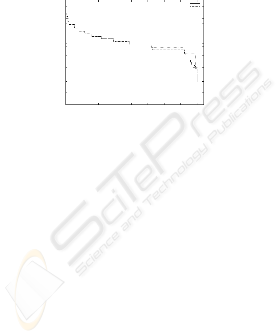
It must be noted that the ﬁne tuning of the above factors is always a compromise

between precision on the one hand and the number of documents for which a cluster

can be generated as well as cluster size on the other. This can be seen in Fig. 2. The

unadjusted level l obviously is an inferior measure. Both of the adjusted levels lie close

to each other, with a slight advantage for l

. This is not too surprising since asymptoti-

cally, they are equal.

The maximum precision that was reached by using l

was 0.95 at level 0.95, but

then, recommendations could only be generated for 11 documents out of nearly 40,000.

113

0.2

0.3

0.4

0.5

0.6

0.7

0.8

0.9

0 5000 10000 15000 20000 25000 30000 35000 40000

0.2

0.3

0.4

0.5

0.6

0.7

0.8

0.9

1.1

precision

number of documents with recommendations

precision l

Fig.2. Precision versus number of documents with a recommendation

On the other hand, in order to have recommendations for more than 50% (26,067 in this

case) of the documents, a precision of 67% is feasible.

A manual evaluation of these results by a human test group is in preparation in order

to verify these ﬁrst results.

6 Conclusion and Outlook

We have presented a new method for generating recommendations on large data sets in

an efﬁcient way. The precision and performance we were able to achieve are promising.

However, there remain some open questions for further research: An important issue

that is currently in the focus of research is that of intelligently updating the clusters

when new usages histories arrive by reusing as much as possible from the existing

walks. Furthermore, a more intelligent decision for the number of walks that are started

from a node will be implemented in order to maximize coverage of the graph without

unnecessarily driving up computation time. For this purpose, it is also important to

better understand the asymptotic behavior of the algorithm as the number of walks

approaches inﬁnity.

Although Sch

oll [17] has tested this clustering method against others in several

typical situations, it will be interesting to perform this comparison also on our library

data or – due to computational complexity – on a subset thereof.

Acknowledgment. We gratefully acknowledge the funding of the project “RecKVK”

by the Deutsche Forschungsgemeinschaft (DFG).

114

References

1. Schafer, J.B., Konstan, J.A., Riedl, J.: E-commerce recommendation applications. Data

Mining and Knowledge Discovery 5 (2001) 115–153

2. Franke, M., Thede, A.: Clustering of Large Document Sets with Restricted Random Walks

on Usage Histories. In Weihs, C., Gaul, W., eds.: Classiﬁcation – the Ubiquitous Challenge,

Heidelberg, GfKl Deutsche Gesellschaft f

ur Klassiﬁkation, Springer (2005) 402–409

3. Resnick, P., Varian, H.R.: Recommender Systems. CACM 40 (1997) 56 – 58

4. Gaul, W., Geyer-Schulz, A., Hahsler, M., Schmidt-Thieme, L.: eMarketing mittels Recom-

mendersystemen. Marketing ZFP 24 (2002) 47 – 55

5. Geyer-Schulz, A., Hahsler, M., Jahn, M.: Educational and scientiﬁc recommender systems:

Designing the information channels of the virtual university. International Journal of Engi-

neering Education 17 (2001) 153 – 163

6. Nichols, D.M.: Implicit rating and ﬁltering. In: Fifth DELOS Workshop: Filtering and

Collaborative Filtering, ERCIM (1997) 28–33

7. Semeraro, G., Ferilli, S., Fanizzi, N., Esposito, F.: Document classiﬁcation and interpretation

through the inference of logic-based models. In P. Constantopoulos, I.S., ed.: Proceedings of

the ECDL 2001. Volume 2163 of LNCS., Berlin, Springer Verlag (2001) 59–70

8. Yang, Y.: An evaluation of statistical approaches to text categorization. Information Retrieval

1 (1999) 69–90

9. Ehrenberg, A.S.: Repeat-Buying: Facts, Theory and Applications. 2 edn. Charles Grifﬁn &

Company Ltd, London (1988)

10. Geyer-Schulz, A., Neumann, A., Thede, A.: An architecture for behavior-based library rec-

ommender systems – integration and ﬁrst experiences. Information Technology and Libraries

22 (2003) 165 – 174

11. Duda, R.O., Hart, P.E., Stork, D.G.: Pattern Classiﬁcation. 2 edn. Wiley-Interscience, New

York (2001)

12. Bock, H.: Automatische Klassiﬁkation. Vandenhoeck&Ruprecht, G

ottingen (1974)

13. Sarwar, B.M., Karypis, G., Konstan, J., Riedl, J.: Recommender systems for large-scale e-

commerce: Scalable neighborhood formation using clustering. In: Proceedings of the Fifth

International Conference on Computer and Information Technology, Bangladesh (2002)

14. Kohrs, A., Merialdo, B.: Clustering for collaborative ﬁltering applications. In: Computa-

tional Intelligence for Modelling, Control & Automation 1999. Volume 55 of Concurrent

Systems Engineering Series., Amsterdam, IOS Press (1999) 199–204

15. Viegener, J.: Inkrementelle, dom

anenunabh

angige Thesauruserstellung in dokument-

basierten Informationssystemen durch Kombination von Konstruktionsverfahren. inﬁx,

Sankt Augustin (1997)

16. Sch

oll, J., Sch

oll-Paschinger, E.: Classiﬁcation by restricted random walks. Pattern Recog-

nition 36 (2003) 1279–1290

17. Sch

oll, J.: Clusteranalyse mit Zufallswegen. PhD thesis, TU Wien, Wien (2002)

18. Sch

oll, J., Paschinger, E.: Cluster Analysis with Restricted Random Walks. In Jajuga, K.,

Sokolowski, A., Bock, H.H., eds.: Classiﬁcation, Clustering, and Data Analysis, Heidelberg,

Springer-Verlag (2002) 113–120

19. Erd

os, P., Renyi, A.: On random graphs I. Publ. Mathematicae 6 (1957) 290–297

20. Kunz, M., et al.: SWD Sachgruppen. Technical report, Deutsche Bibliothek (2003)

115