STEREO IMAGE BASED COLLISION PREVENTION USING THE

CENSUS TRANSFORM AND THE SNOW CLASSIFIER

Christian K

ublbeck, Roland Ach, Andreas Ernst

Fraunhofer Institute for Integrated Circuits

Am Wolfsmantel 33

Keywords:

stereo, obstacle detection, census transformation, SNoW classiﬁer.

Abstract:

In this paper we present an approach for a mobile robot to avoid obstacles by using a stereo-camera system

mounted on it. We use the “census transformation” to generate the features for the correspondence search. We

train two SNoW (Spare Network of Winnovs)-classiﬁers, one for the decision wether to move straight forward

or to evade and a second one for deciding whether to turn left or right when evading. For training we use a

sample set collected by manually moving around with the robot platform. We evaluate the performance of the

whole recognition chain (feature generation and classiﬁcation) using ROC-curves. Real world experiments

show the mobile robot to safely avoid obstacles. Problems still arise when approaching steps or low obstacles

due to limitations in the camera setup. We propose to solve this problem using a stereo camera system capable

of pan and tilt movements.

1 INTRODUCTION

The detection of obstacles is an important research

topic in the ﬁeld of autonomous robots. Collisions

have to be avoided, since robots must neither endan-

ger human beings through their movement nor dam-

age themselves or objects in the environment. The

aim of the present work is to develop a system for

obstacle detection and collision avoidance for an au-

tonomous robot with the aid of a stereoscopic camera

setup. Further on aiming at a later 3D-map genera-

tion of the environment an unsupervised exploration

trip through a building should be permitted. For that

purpose appearing obstacles like walls, objects or per-

sons must be detected.

1.1 Overview

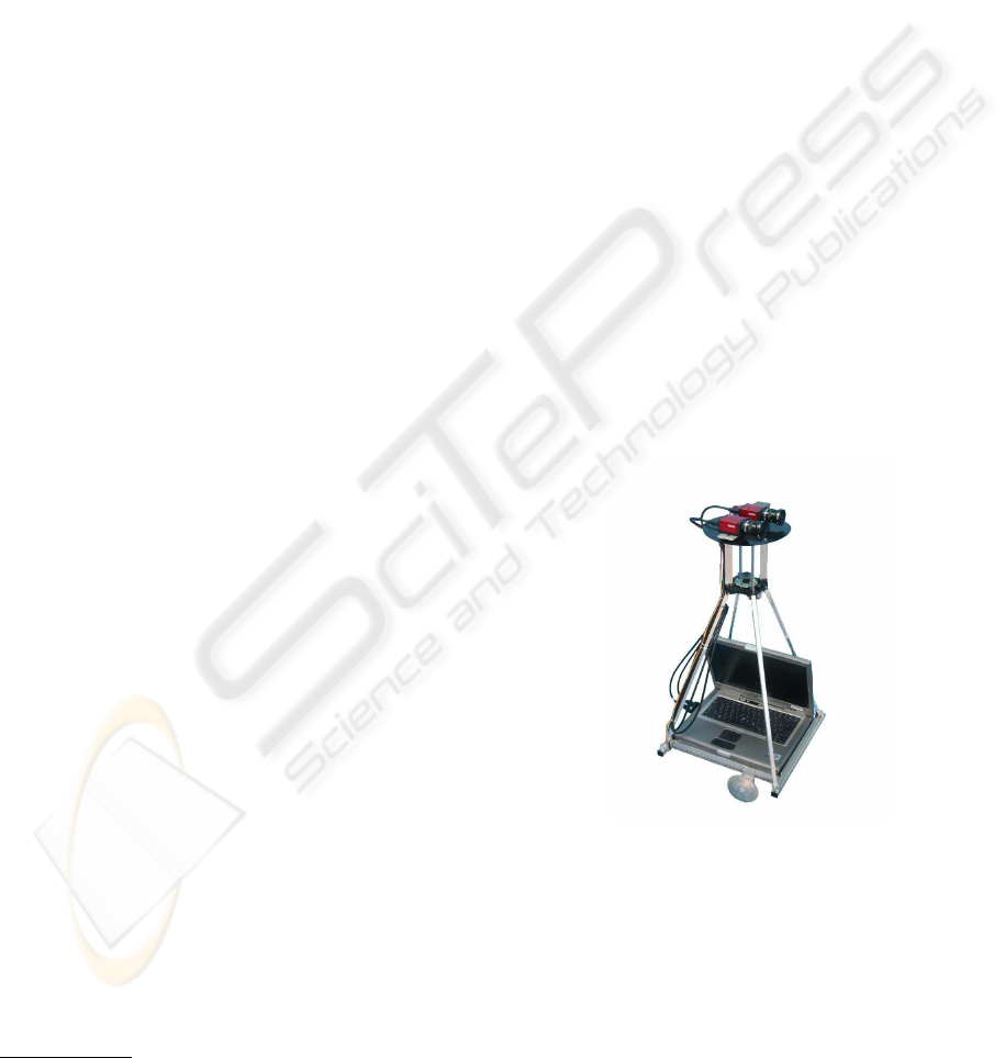
The robot is based on a mobile platform named Volks-

Bot

that consists of a main frame with the dimen-

sions 40 x 40 x 80 cm. The drive mechanism is made

up of two DC-motors with 22 W power and 24 V

nominal voltage. The two drive wheels forms a tri-

angle together with a third rear wheel. On the lower

The VolksBot has been developed by the Fraunhofer In-

stitute for Autonomous Intelligent Systems AIS in Sankt

Augustin, Germany.

Figure 1: The robot based on the mobile platform VolksBot.

platform a standard notebook with an 1.6 MHz mo-

bile processor is placed. The communication with the

motor controller is established by the serial RS232-

Interface.

For stereo image capturing, we use two ﬁrewire

cameras. They are mounted parallel to each other on

a small upper platform at a height of 80 cm. The op-

tical axes are arranged in a distance of approximately

447

Küblbeck C., Ach R. and Ernst A. (2005).

STEREO IMAGE BASED COLLISION PREVENTION USING THE CENSUS TRANSFORM AND THE SNOW CLASSIFIER.

In Proceedings of the Second International Conference on Informatics in Control, Automation and Robotics - Robotics and Automation, pages 447-454

DOI: 10.5220/0001184804470454

 SciTePress

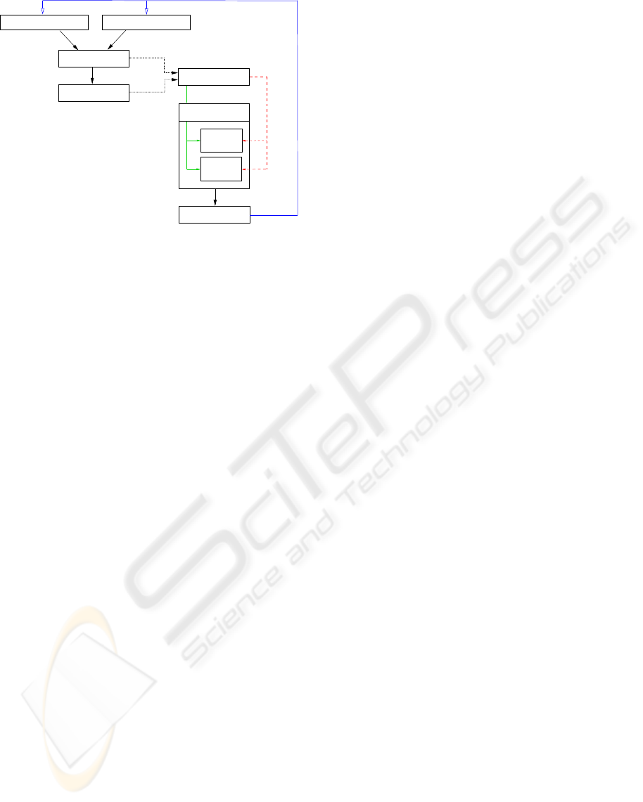
Image from right Camera

Train

Image from left Camera

Depth Map

Disparity Image

Obstacle

Classifier

Direction

Classifier

Classify

Feature Extraction

Robot Drive

State Machine

Figure 2: System structure.

10 cm. Both cameras are equipped with a wide angle

lens with 4.2 mm of focal length.

Figure 2 shows the structure of the system setup.

Two cameras are used for image capturing. We are

scaling down the images to a size of 320 x 240 pix-

els and only use one single color channel. A pair of

images is grabbed approximately every 240 ms. Thus

about four frames per second are processed. In or-

der to extract depth-information, a disparity image is

determined by means of block matching. To reduce

noise artifacts smoothing ﬁlters like mean or median

are applied to the original images. Additionally we

use the census transform to get suitable images for

the subsequent block matching. Using a lookup table

derived from the camera geometry, we can calculate

a depth map from the disparity image. These results

serve as the basis for the feature extraction. Hence the

complete disparity image or depth map can be used. It

is also possible only to use the distance of the nearest

obstacle for each picture column of the depth map.

Alternatively height information of the objects situ-

ated in the area can be included.

Based on the classiﬁcation results the robot is con-

trolled in its movements. We are using two state ma-

chines. Therefore, two classiﬁers are integrated. The

ﬁrst one recognizes obstacles that have to be avoided.

If an obstacle is detected, the second classiﬁer is

asked for a preferred evasive direction. This direc-

tion is retained until a movement straight forward is

possible again.

1.2 State of the Art

Most solutions of obstacle avoiding robots use laser

range sensors, ultrasonic or infrared sensors, but there

are also realizations using cameras. Especially 2-

camera-systems often serve as a basis for the obstacle

detection.

In this sense, Kumano, Ohya and Yuta

(Masako Kumano and Yuta, 2000) follow a very sim-

ple approach. Using two cameras directed in a ﬁxed

angle towards the ground, images of the environment

are obtained. Starting from the geometrical setup

between the cameras and the ﬂoor, corresponding

points in both images are determined. Intensity

differences between corresponding points in both

images are assumed to be an obstacle in the way. The

scan lines correspond to different distances according

to the camera arrangement. Evaluating merely three

scan lines that represent the distances 40 cm, 65 cm

and 100 cm, a fast computing time (35 ms) can be

guaranteed.

Sabe, Fukuchi, Gutmann, Ohashi, Kawamoto and

Yoshigahara (Kohtaro Sabe et al., 2004) also use two

CCD-cameras. These are integrated in the humanoid

Sony QRIO Robot. Firstly landmark points of the en-

vironment are searched in both images. These points

appear in different picture coordinates according to

the different camera views and the distance. Using

these disparities, 3D coordinates can be computed.

On this basis the robot detects possible obstacles on

the ﬂoor level, that are used for path planning.

The electrical wheelchair Victoria (Libuda and

Kraiss, 2004) computes a depth map from the in-

cluded scene with the aid of a camera pair. Additional

corners and edges are determined in different detec-

tion stages and grouped to regions which correspond

to certain objects in the room. Using ﬁxed relations

between these landmarks a model of the surroundings

can be produced with the corresponding distance in-

formation. One can search the walls for regions like

doors and the ﬂoor for obstacles.

There is still a number of further approaches with

two camera systems. For example the NEUROS

project at the Ruhr University of Bochum with its

visually controlled service robot Arnold uses such

a construction (Ruhr-Universit

at, 1997). Arnold ex-

tracts edges from both images and calculates their dis-

tances by the shift of these landmarks. Hence apart

from an obstacle detection, card generation of the en-

vironment is possible. In unknown areas the robot

turns by 360 degrees to get the necessary data. To

evade people optical ﬂow is included.

Another example is the Ratler (robotic all terrain

lunar exploration rover) (Reid Simmons and Whelan,

1996). It moves in an unknown area with a height-

map of the environment. This map is generated by the

extraction of 3D-points from a stereo-camera-system.

Daimler Chrysler develops a system for the detec-

tion of pedestrians (D.M. Gavrila and Munder, 2004).

At ﬁrst a disparity image indicates potential areas. By

an edge extraction of these regions a comparison with

sample forms of persons is possible.

ICINCO 2005 - ROBOTICS AND AUTOMATION

448

Baseline b

optical axis

M ( x , y , z )

− u

r r

m ( u , v )

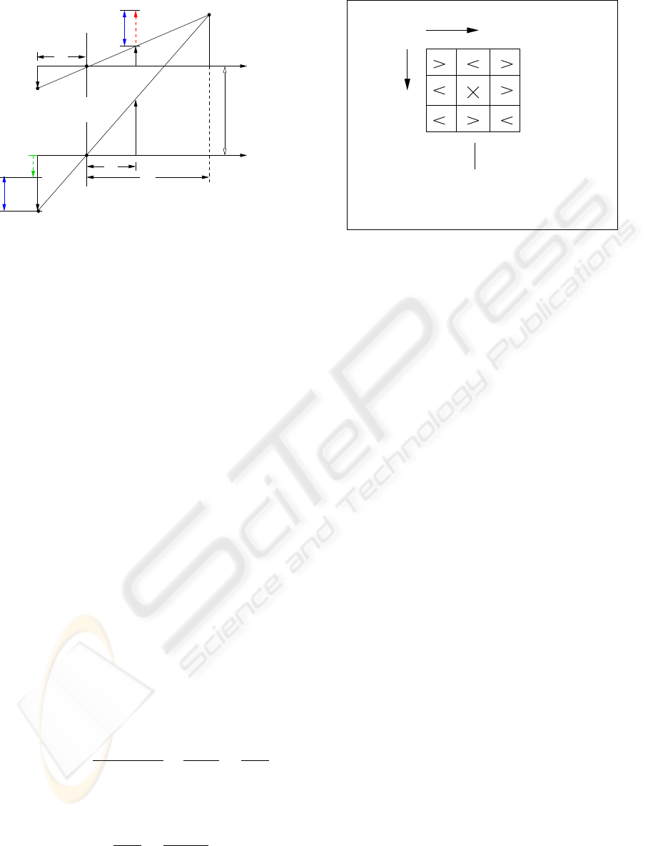
Figure 3: Simple model of the stereo camera system.

2 FEATURE GENERATION

2.1 Camera Setup and Stereo

Geometry

A standard camera projects three-dimensional objects

of the real world onto the 2D image plane. A very

simple model of this process is given by the pinhole

camera. In this case the optic consists of one inﬁnitely

small hole.

A simple possibility to recover depth information

of the captured scene is an extension of a single cam-

era by a second identical camera with same focal

length. The visual axes of both cameras are arranged

in parallel and on the same level. In ﬁgure 3 a point M

of the real world is projected to different coordinates

, v) and m

, v) on the image planes because

of the varying camera viewpoints. The difference is

called disparity d. Using the knowledge about the

geometrical camera setup and the focal length f the

distance z

of the point M from the camera plane can

be computed by means of the disparity. It is inversely

proportional to the distance.

Depending on the distance b of the two camera axis

the following relations can be derived from the stereo-

geometry:

d = u

− u

f ∗ (x

+ b)

−

f ∗ x

f ∗ b

. (1)

Using the disparity d the distance z

can therefore

be computed by

f ∗ b

− u

. (2)

The standard stereo geometry assures that arbitrary

points of the 3D scene are always projected into the

CensusVector 101 01 010

Neighborhood

Pixel

Image

Scanning

Figure 4: The census transform: Each pixel is compared

with its eight neighbours. From the binary results of the

comparisons a feature of one byte is constructed.

same line in both images. For this reason only hor-

izontal disparities appear. This restriction is called

epipolar constraint. Hence the search area ﬁnding

corresponding points in both image planes can be re-

duced to one dimension.

It is important to mention that disparities can be

determined only for points from objects that can be

observed in both images. With increasing camera dis-

tance b this overlap becomes smaller.

2.2 The Census Transform

In order to compute disparity informations it is nec-

essary to ﬁnd corresponding points in both images.

It has to be considered, that the internal attitudes of

the two cameras can differ, regarding gain and biases.

Therefore corresponding regions may have different

absolute intensities. To solve this problem we use the

census transform proposed by Zabih and Woodﬁll. It

offers a brightness invariant comparison possibility.

Additionally it provides an efﬁcient and fast methods

to extract features for structured image regions that

can serve as feature points.

The census transform compares each pixel with its

eight neighboring pixels. If the intensity of the center

is greater, the appropriate bit of the census feature is

set, otherwise cleared. Therefore the census feature

has eight bit and can be used to represent a grey tone

in a new “census-image”. The shift of the window

over the entire image results in a complete census im-

age. This procedure is applied to both camera images.

The distance between two census features can be

computed using the hamming distance. It is calcu-

lated by counting the number of bits that differ within

both census features.

To ﬁnd corresponding points for each area of the

STEREO IMAGE BASED COLLISION PREVENTION USING THE CENSUS TRANSFORM AND THE SNOW

CLASSIFIER

449

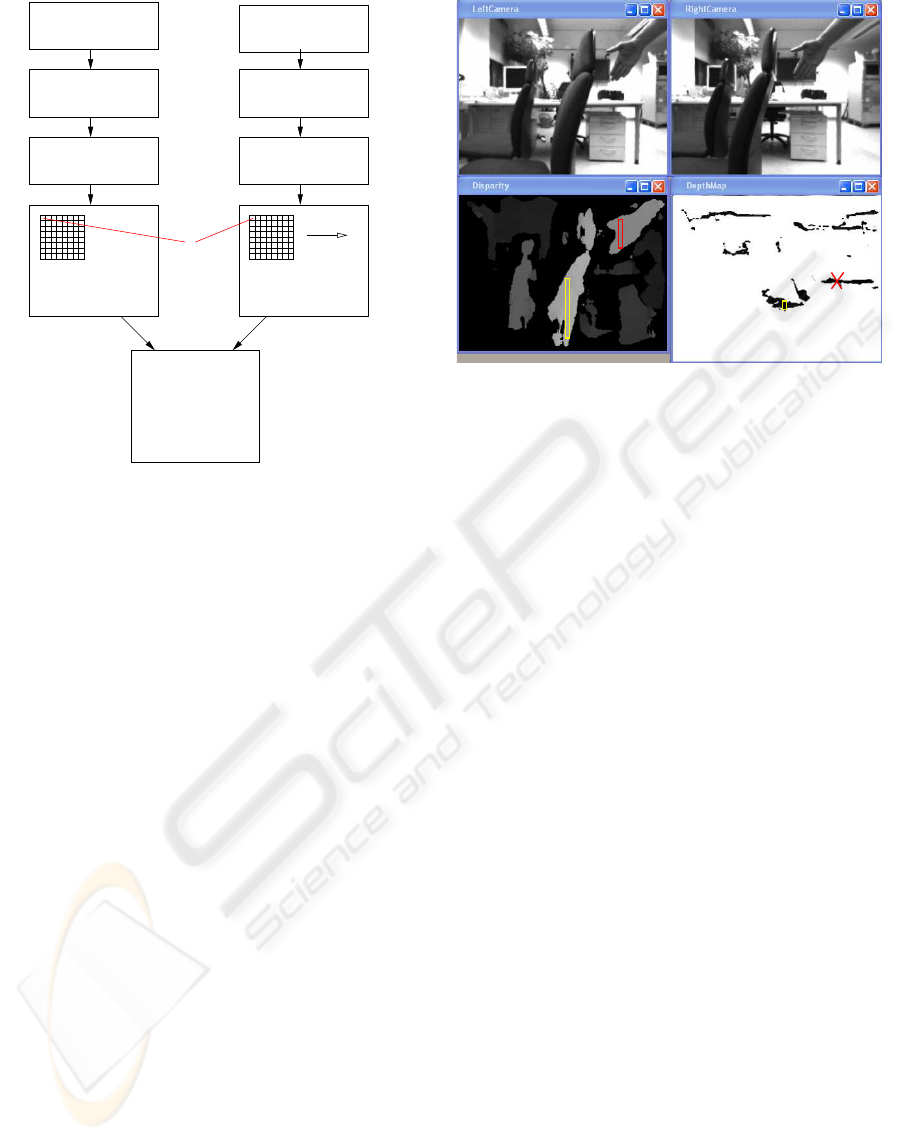
Image from left Camera

Mean / Median

Census transformation

Census Image

Census transformation

Census Image

Disparity Image

Image from right Camera

Mean / Median

HammingDistance

Figure 5: Generation of the disparity image.

ﬁrst census image every point is compared to each

region in the second census image within the same

image line. The hamming distance between all pairs

of points is calculated and summed up for the com-

plete area. The minimum distance for each pixel cor-

responds to the most similar picture region.

2.3 Generation of Disparity Maps

and Features

As ﬁgure 5 shows, the original camera images are

ﬁltered at the beginning of the process, alternatively

with a mean or median ﬁlter of size 3 × 3. Then the

census transform is used to ﬁnd corresponding pixels

in both images.

To generate the disparity image a block matching

procedure is used. This method takes a pixel neigh-

borhood to ﬁnd similar areas. The size of this region

is parameterizable.

The best disparity is estimated at the points where

the hamming distance reaches its minimum. Addi-

tionally the applied algorithm uses a so-called conﬁ-

dence procedure which describes the reliability of the

estimation. This is done by computing ﬁrstly the ham-

ming distance at the estimated disparity and the aver-

age of discrete similarity values obtained shifting the

window along the image line. If the distance between

both is smaller than a ﬁxed conﬁdence threshold the

result is discarded and the appropriate pixel in the dis-

parity picture is set to zero. This method affects par-

ticularly weakly textured, homogeneous areas where

Figure 6: Disparity image and depth map.

wrong assignments occur rather often. Figure 6 shows

an example of a disparity image. Brighter parts of the

image correspond to closer ranges, dark regions be-

long to more distant objects in the scene.

From the disparity image a kind of bird’s eye view

of the captured scene can be generated by summing

up the existing disparity values for each column ac-

cording to their occurrence by registering them in a

depth map. The y-axis represents the disparities, the

x-axis the picture column. The value contains infor-

mation about the vertical expansion of the objects.

The objects can be found according to their order in

the depth map. With help of the stereo geometry and

equation 2 the distance can be determined in real met-

ric numbers. So the two ofﬁce chairs are about 54

cm and 104 cm away from the cameras. The hand

is found approximately 69 cm in front of the camera.

As we will see later this knowledge is not necessary

for our approach. The critical distance for objects in

front of the robot is implicit given by the disparities

of the training data containing an obstacle. Of course

the reliability of the depth map strongly depends on

the quality of the disparity image.

Human beings are able to recognize directly from

the depth map whether an obstacle is in a critical

range. In opposite a computer has to perform an addi-

tional preprocessing step for feature extraction prior

to the classiﬁcation. For this purpose a very simple

approach is coding the respective pixels of the dis-

parity image or depth map with coordinates and grey

tones in a characteristic feature vector. Of course the

feature vector and each feature respectively, depen-

dent on the dimensions of the image, can become very

large. In order to handle these data the images can be

scaled down. On basis of a size of 320 × 240 a re-

duction to 80 × 60 makes sense. Besides the above

ICINCO 2005 - ROBOTICS AND AUTOMATION

450

Distance Contour from DepthMap

Complete Disparity− or Depthmap

Pixel ( 0 , 0 )

Pixel ( 0 , Distance ) Pixel ( Width , Distance )

Pixel ( Width , Height )

Column Distance

Intensity

X X

Disparity DisparityYY

Figure 7: Possible encodings of the feature vectors.

x 2

F 1

y 1

C s

F 2

SNOW

y 2

y 1 − y 2

x n

FeatureVector TargetNodesInputNodes

x 1

w1n

w21

w2n

w11

Figure 8: Architecture of the SNoW-classiﬁer

rather simple approach it is also possible to use only

one value representing the nearest obstacle for each

column of the depth map. With respect to the whole

image pair thus a distance contour of the objects arises

from the ﬁeld of vision of the robot. Figure 7 illus-

trates both methods of feature encoding.

3 CLASSIFICATION WITH SNOW

The classiﬁcation has to categorize a characteristic

feature vector by comparison with reference samples.

Due to the very complex features a neural network

which can build high-dimensional separation func-

tions between the individual classes is used. In this

work we use a special network named SNoW (Sparse

Network of Winnows)(Yang et al., 2000). The SNoW

is characterised by high detection achievement and

speed. Therefore it is used in speech processing or

in the ﬁeld of face detection. In this case the classi-

ﬁer has to decide between the classes ’forward’, ’turn

left’ and ’turn right’. Hence, two classiﬁers are used.

The ﬁrst one decides between free and obstacle, the

second one suggests a suitable evasive direction if it

is necessary.

The architecture of the network consists of a layer

of input nodes and a layer of target nodes. One target

node represents a special class. Both levels are con-

nected by weighted edges. The number of input nodes

Feature 1

Feature 4800

21 Bit

Decimal 68

7 Bit

1 1

0000000

000000

01000100

1001111

00110001

111011

1309489

Decimal 1309489

8 Bit6 Bit7 Bit 6 Bit

8 Bit

2^21−1

= 2097151

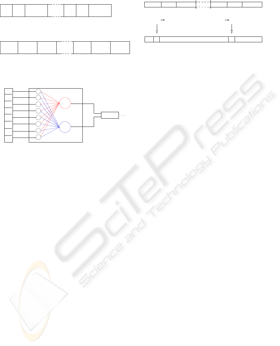
Figure 9: SNoW-feature vector

depends on the binary representation of the charac-

teristic feature vectors. Figure 9 shows such a struc-

ture for a pixel-coded depth map with a dimension of

80×60 pixels. The vector length depends on the num-

ber of bits per feature: length = 2

bits per feature

. In this

case each feature represents a position within the vec-

tor according to its binary value. In these places the

vector takes the value ’1’. The remaining positions

are set to ’0’.

Vector entries with the value 1 are called active

characteristics. Only these components are attached

over weights to the target nodes t. The activation F

of these elements is determined over the sum of the

connected weights according to equation 3. However,

these nodes are active only if their activations exceed

a certain class threshold Θ

< F

i∈A

(3)

here is the amount of all active features i con-

nected to the node t: A

= {i

, ..., i

} .

The weights are at ﬁrst uniformly determined. Dur-

ing the training phase an adjustment takes place only

if a false classiﬁcation happens. The update strategy

is based thereby on a promotion parameter α > 1 for

increasing and a demotion parameter 0 < β < 1 for

reducing the values.

With well-known input vectors

t for the class t and

the quantity of the active features m

the following

relationships are established:

t = t and F

) ≤ Θ

: ∀

∈ A

: w

← α∗w

(4)

t 6= t and F

) ≥ Θ

: ∀

∈ A

: w

← β∗w

(5)

The values supplied by each target node, also called

scores are charged with each other. Given that we

only have two-category problems the afﬁliation is car-

ried out using the score difference c = F

− F

. So a

special decision instance is used that can be parame-

trized with a threshold. Thus a sensitivity regulation

for a certain class becomes feasible.

STEREO IMAGE BASED COLLISION PREVENTION USING THE CENSUS TRANSFORM AND THE SNOW

CLASSIFIER

451

if ( FREE )

if ( OBSTACLE )

Classifier

Ask Obstacle

Ask Direction

if ( OBSTACLE )

Turn RightDrive Forward

if ( FREE )

Turn Left

if ( OBSTACLE )

if ( LEFT ) if ( RIGHT )

Figure 10: State machine.

The decision for class 1 is made if c +

Sensitivity > 0 and similarly the decision for class

2 is made if : c + Sensitivity ≤ 0

In order to guide the robot, control commands must

be sent to the motor controller permanently. The co-

ordination of these instructions needs a state machine

presented in ﬁgure 10. This machine is in one of

the three possible states ’forward’, ’turn left’ or ’turn

right’ at each time. The transitions are ﬁxed exactly

and are followed according to the appearing events.

Each instance contains one SNoW-classiﬁer for the

obstacle detection and one for the direction decision,

respectively. At the beginning an image pair is ex-

amined and it is decided, whether an obstacle is in

front of the robot. If this is true the second classiﬁer

is asked about a suitable evasive direction. The unity

therefore represents the condition ’turn left’ or ’turn

right’. This decision has to be maintained until the

obstacle detector indicates a free way again. Then the

machine again represents the condition ’forward’.

4 EXPERIMENTS AND RESULTS

The training data was collected by controlling the ro-

bot manually. Normally the robot moves straight on.

If there is an obstacle in front of it a change of di-

rection can be enforced by pressing the left or right

mouse button depending on the best way to elude.

This movement is maintained till the button is re-

leased. In this case the vehicle goes straight on again.

During the complete journey the system saves the

two current camera images on hard disk. This hap-

pens approximately at a rate of ﬁve frames per sec-

ond. The size of the images is 320 × 240 pixel using

only grey level format. Hence the ﬁle size is reduced

to about 40 kB. In order to mark obstacles the ﬁle-

name consists of a time stamp and the current control

information like forward, left or right.

This way approximately 100,000 training images

were recorded. 39552 pairs correspond to the class

’forward’, 9342 couples containing obstacles. To ﬁnd

alternate directions 4788 pairs represent turns to the

0.0 0.2 0.4 0.6 0.8 1.0

0.0

0.6

0.2

0.4

0.8

1.0

Sensivity

1 − Specificity

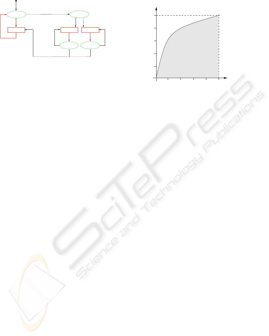
Area Under Curve

Figure 11: ROC-curve.

left, 4554 turns to the right. This data is grouped

in two different lists. On the one hand all ﬁles are

taken up to an obstacle list, whereby the classes ’turn

left’ and ’turn right’ correspond to an obstacle. On

the other hand a direction list covers all image pairs

which are not part of the class ’forward’. These two

lists are used for the training of the obstacle classiﬁer

and direction classiﬁer respectively.

Depending on preprocessing and feature extraction

the training takes up to eight hours on standard hard-

ware (with a 1.5 GHz processor). Both classiﬁers

are trained separately. For evaluation purposes fur-

ther test data has been collected. It consists of 14447

image pairs divided in 13119 with the label ’for-

ward’, 790 of the class ’turn left’ and 538 of the class

’turn right’. By comparison of the well known class

memberships with the classiﬁcation result a statement

about the quality of the trained classiﬁers can be met.

With the search for a proved decision criteria for

the optimization of the preprocessing and feature ex-

traction parameters like block size, search width, con-

ﬁdence threshold, mean or median ﬁltering of the

depth map, etc. the choice felt on the so-called ROC

curve. The ROC method applies the fraction of cor-

rect classiﬁed obstacles to the y-axis of a diagram. On

the x-axis the ratio of wrong classiﬁed free areas is

registered. These informations are based on sample

data. Figure 11 shows a sample ROC curve. The ap-

pearance of the curve is based on different decision

borders. On the left side the curve starts with a very

high separative work. One surveys everything, how-

ever no images of the class ’forward’ were classiﬁed

falsely as an obstacle. The lowest decision limit lies

on the right side. One does not survey anything, since

one categorizes all inputs as obstacle. In view on the

choice of these separative borders it is necessary to

look on the scores determined by the obstacle classi-

ﬁer for both classes.

The area below the curve is a measure for the qual-

ICINCO 2005 - ROBOTICS AND AUTOMATION

452

0.2

0.4

0.6

0.8

0 0.2 0.4 0.6 0.8 1

Detection rate (DET)

False acceptance rate (FAR)

Best DisparityMap

Best DepthMap

Best Distance Vector

Best Distance Vector with Height

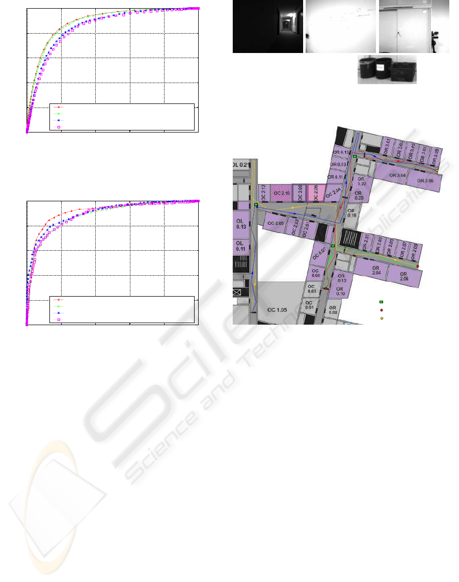
Figure 12: ROC-curves for obstacle classiﬁer.

0.2

0.4

0.6

0.8

0 0.2 0.4 0.6 0.8 1

Detection rate (DET)

False acceptance rate (FAR)

Best DisparityMap

Best DepthMap

Best Distance Vector

Best Distance Vector with Height

Figure 13: ROC-curves for direction classiﬁer.

ity of the classiﬁer. The curve ideally arises vertically

up on the left. So the curve forms a square of area

1 with the coordinate axes. The area under the ROC

curve serves as a criterion for the improvement of the

adjusted parameters. The more this value reaches 1,

the better a separation into the two classes is possible.

Like the obstacle classiﬁer, the direction classiﬁer

uses the ROC method to optimize the parameters.

Based on sample images correct classiﬁed pictures of

the class ’turn left’ lay over wrongly assigned pictures

of the class ’turn right’.

Despite all improvement some pairs of images

from the sample are still categorized falsely. Exam-

ining more closely these images makes clear, that the

majority of wrong classiﬁed samples are quite prob-

lematic. Some pictures are almost without any light-

ing. Furthermore reﬂecting surfaces or images with

sparse texture (for example white walls) cause cer-

tain difﬁculties. The main problem however lies in

the cameras mounted parallel to the ground. Since

they are ﬁxed at the height of 80 cm smaller objects

on the ﬂoor are not in the ﬁeld of view and therefore

Figure 14: Examples of wrong classiﬁed images.

Problem with glass door

Start / End

Obstacle

Figure 15: Travel through a building.

cannot be detected. During the generation of test data

by means of a mouse control the evade of these ob-

stacles is guaranteed by the supervisor. But these ob-

jects are not seen within the image. So the classiﬁer

is not able to make the right decision. For this reason

the cameras should be operated looking to the ground.

Figure 14 shows some examples of wrong classiﬁed

images.

5 CONCLUSION AND OUTLOOK

Figure 15 represents as an example a travel of the ro-

bot through our institute building. The best classi-

ﬁers are used. Problems occured only in front of glass

doors.

In order to make the system more robust, the cam-

eras should be installed with view to the ground. The

optimum would be a mobile camera head. Its ad-

justment could be included in the feature vectors too.

Thus also smaller objects could be detected such as

legs of a chair or boxes standing on the ﬂoor. At the

current setup smaller objects disappear when moving

STEREO IMAGE BASED COLLISION PREVENTION USING THE CENSUS TRANSFORM AND THE SNOW

CLASSIFIER

453

towards them in critical distances.

Furthermore sequences with different lighting con-

ditions or shades could be generated to consider these

inﬂuences particularly. Also a speed control could be

installed by mapping the score differences of the ob-

stacle classiﬁer. The robot could accelerate if no ob-

stacles are seen and slow down if objects are near. At

collisions an image sequence could be saved to retrain

and improve the classiﬁer after the event.

REFERENCES

D.M. Gavrila, J. G. and Munder, S. (2004). Vision-based

pedestrian detection: The protector system. Daimler

Chrysler Research , Ulm.

Kohtaro Sabe, Masaki Fukuchi, J.-S. G., Ohashi, T.,

Kawamoto, K., and Yoshigahara, T. (2004). Obsta-

cle avoidance and path planning for humanoid robots

using stereo vision. Sony Corporation, Tokyo.

Libuda, L. and Kraiss, K.-F. (2004). Identiﬁcation of nat-

ural landmarks for vision based navigation. Technis-

che Universit

at Aachen.

Masako Kumano, A. O. and Yuta, S. (2000). Obstacle

avoidance of autonomous mobile robot using stereo

vision sensor. University of Tsukuba.

Reid Simmons, Lars Henriksen, L. C. and Whelan, G.

(1996). Obstacle avoidance and safeguarding for a lu-

nar rover. Carnegie Mellon University.

Ruhr-Universit

at, B. (1997). Arnold, ein autonomer

service-roboter. http://www.neuroinformatik.ruhr-

uni-bochum.de/ini/PROJECTS/NEUROS/ff97-

katalog/arnold

d.html.

Yang, M.-H., Roth, D., and Ahuja, N. (2000). A snow-

based face detector. In Advances in Neural Informa-

tion Processing Systems 12 (NIPS 12), pages 855–

861. MIT Press.

ICINCO 2005 - ROBOTICS AND AUTOMATION

454