ON TEMPORAL DIFFERENCE ALGORITHMS

FOR CONTINUOUS SYSTEMS

Alexandre Donz

Verimag Laboratory

2 avenue de Vignate, 38100 Gi

eres, France

Keywords:

Optimal Control of Continuous Systems, Dynamic Programming, Optimal Value function, Reinforcement

Learning, Temporal Differences Algorithms.

Abstract:

This article proposes a general, intuitive and rigorous framework for designing temporal differences algorithms

to solve optimal control problems in continuous time and space. Within this framework, we derive a version

of the classical TD(λ) algorithm as well as a new TD algorithm which is similar, but designed to be more

accurate and to converge as fast as TD(λ) for the best values of λ without the burden of ﬁnding these values.

1 INTRODUCTION

Dynamic programming (DP) is a powerful technique

to compute optimal feedback controllers which was

developed at the early stages of the ﬁeld of optimal

control (Bellman, 1957). It has been used since then

in a wide variety of domains ranging from control

of ﬁnite state machines, Markov Decision Process

(MDP), to optimal control of continuous and hybrid

systems. For all these problems, its goal is to compute

a so-called value function (VF) mapping the states of

the system to numbers that reﬂect the optimal cost to

reach a certain objective from these states. Once this

function computed, the optimal feedback control can

be easily deduced from its values. The main draw-

back of DP lies in its computational cost. Computing

the VF over the whole state space of the system can

be prohibitively expensive if the number of states is

large, particularly if it is inﬁnite, e.g. in the case of

continuous problems. This led some to develop re-

laxed DP techniques, e.g. (Rantzer, 2005).

In the reinforcement learning (RL) community,

the temporal difference (TD) family of algorithms

gained a particular interest after several spectacular

experimental success, such as TD-Gammon (Tesauro,

1995), a player of backgammon that outperformed

professional human players. These algorithms work

by “learning” the VF while observing simulated tra-

jectories. This family of algorithms is most typ-

ically designed for discrete MDPs, but various at-

tempts were also made to adapt it to optimal control

of continuous systems, see (Sutton and Barto, 1998)

for a survey. Recently, one of these works gave very

promising and impressive results in the control of a

continuous mechanical system with a large number of

degrees of freedom and input variables (respectively

14 and 6) (Coulom, 2002). This motivated our in-

terest in studying the applicability of TD algorithms

to continuous optimal control problems. The main

problem of this study is the lack of theoretical results

such as convergence proofs, uniqueness of solutions

and so on. For TD algorithms, results are generally

available in their original context of MDPs and are

not trivial to adapt to the continuous case. On the opti-

mal control side, the most advanced theoretical frame-

work available is that of functional analysis applied

to the numerical solutions of Hamilton Jacobi Bell-

man (HJB) equations. To the best of our knowledge,

the most complete and rigorous analysis of RL algo-

rithm in this context is (Munos, 2000), but it does not

include TD algorithms. Algorithms under study are

numerical schemes usually used to solve partial dif-

ferential equations: ﬁnite differences, ﬁnite elements,

etc. Apart from their ease of implementation, one po-

tential advantage of TD methods over other numerical

schemes to compute the solution of HJB equations is

that as it is based on simulation of real trajectories, it

takes into account the structure of the reach set of the

system. Hence, the approximation of the VF will then

naturally converge faster in the ‘interesting’ zones in-

side the reach set. If the optimality is not the prior

objective, the correct exploitation of this feature can

Donzé A. (2005).

ON TEMPORAL DIFFERENCE ALGORITHMS FOR CONTINUOUS SYSTEMS.

In Proceedings of the Second International Conference on Informatics in Control, Automation and Robotics, pages 55-62

DOI: 10.5220/0001183700550062

 SciTePress

allow to design more rapidly a sub-optimal controller

that meets the desired speciﬁcations.

This article attempts to provide a clariﬁed frame-

work for TD algorithms applied to continuous prob-

lems. Our hope is that by clearly identifying and iso-

lating different problems arising in the design of TD

algorithms, it will help to develop new and better TD

algorithms, and to analyze their behavior more rigor-

ously. Our ﬁrst result in this direction is the derivation

of a version of the classical TD(λ) algorithm along

with a new TD algorithm, we called TD(∅), designed

to be more accurate and to converge as fast as TD(λ)

for the best values of λ without the burden of ﬁnding

these values. The works closest to this one are (Doya,

1996), (Doya, 2000) and (Coulom, 2002). Apart from

the TD(∅) algorithm, a contribution w.r.t. these works

is a slightly higher level of abstraction, which allows

an easier intuitive interpretation of the behaviour of

TD algorithms and the role of their parameters, in par-

ticular the λ parameter. It is this interpretation of the

role of λ that led to the design of TD(∅) algorithm.

The paper is organized as follows. Section 2 re-

calls the principles of DP, ﬁrst applied to the sim-

ple case of deterministic discrete transition systems,

then adapted to continuous problems. Section 3 intro-

duces our continuous framework for TD algorithms,

the TD(λ) algorithm instantiated in this framework

and our variant TD(∅). Section 4 present some ex-

perimental results obtained on two test problems.

2 DYNAMIC PROGRAMMING

2.1 DP For Discrete Systems

We ﬁrst consider in this section a purely discrete de-

terministic system with a state set X , an input or ac-

tion set U and a transition map →: X × U 7→ X .

For each pair (x, u) of state-action, a bounded, non-

negative cost value c(x, u) reﬂects the price of tak-

ing action u from state x. Given a state x

and an

inﬁnite input sequence u = (u

), we can thus de-

ﬁne the cost-to-go or value function of the trajectory

→ x

→ . . . as:

) =

∞

n=0

c(x

, u

) (1)

where γ is a discount factor lying strictly between 0

and 1, which prevents the inﬁnite sum V

from di-

verging. Since V

) represents the cost of apply-

ing the input sequence u from x

, the optimal control

problem consists in ﬁnding a sequence u

∗

that mini-

mizes this cost, i.e. V

∗

) ≤ V

), ∀u ∈ U

Note that V

∗

) does not depend on u

∗

and thus

will be noted V

∗

). Instead of searching an optimal

sequence, DP aims at computing directly the optimal

value function V

∗

(x) for all x ∈ X . It relies on Bell-

man equation satisﬁed by V

∗

which is easily deduced

from (1):

∗

(x) = min

u, x

→x

′

c(x, u) + γV

∗

′

) (2)

Once V

∗

has been computed, an optimal sequence u

∗

is obtained by solving the right hand side of Bellman

equation, which gives the state feedback controller:

∗

(x) = arg min

u, x

→x

′

c(x, u) + γV

∗

′

) (3)

Since (2) is a ﬁx point equation, V

∗

can be computed

using ﬁx point iterations. This gives the following

value iteration algorithm. Convergence of this algo-

Algorithm 1 Value Iteration

1: Init V

, i ← 0

2: repeat

3: for all x ∈ X do

4: V

i+1

(x) ← min

u, x

→x

′

c(x, u) + γV

′

)

5: end for

6: i ← i + 1

7: until V has converged

rithm is guaranteed by the discount factor γ which

makes the iteration a contraction. Indeed, it is easy to

see that

i+1

− V

∞

≤ γkV

− V

i−1

∞

2.2 DP in Continuous Time and

Space

In this section, we adapt the previous algorithm to the

continuous case. Let X and U now be bounded sub-

sets of R

and R

respectively, and f : X ×U 7→ R

the dynamics of the system, so that for all t ≥ 0,

˙x(t) = f (x(t), u (t)) (4)

Cost and cost-to-go functions have their continuous

counter parts: for each x and u, c(x, u) is a non-

negative scalar bounded by a constant

c > 0, and for

any initial state x

and any input function u(·),

u(·)

) =

∞

−s

c(x(t), u(t))dt

Where x(t) and u(t) satisfy (4) with x(0) = x

. The

optimal value function, still not depending on u(·), is

such that ∀x ∈ X ,

∗

(x) = min

u(·)∈U

∞

−s

c(x(t), u(t))dt

ICINCO 2005 - INTELLIGENT CONTROL SYSTEMS AND OPTIMIZATION

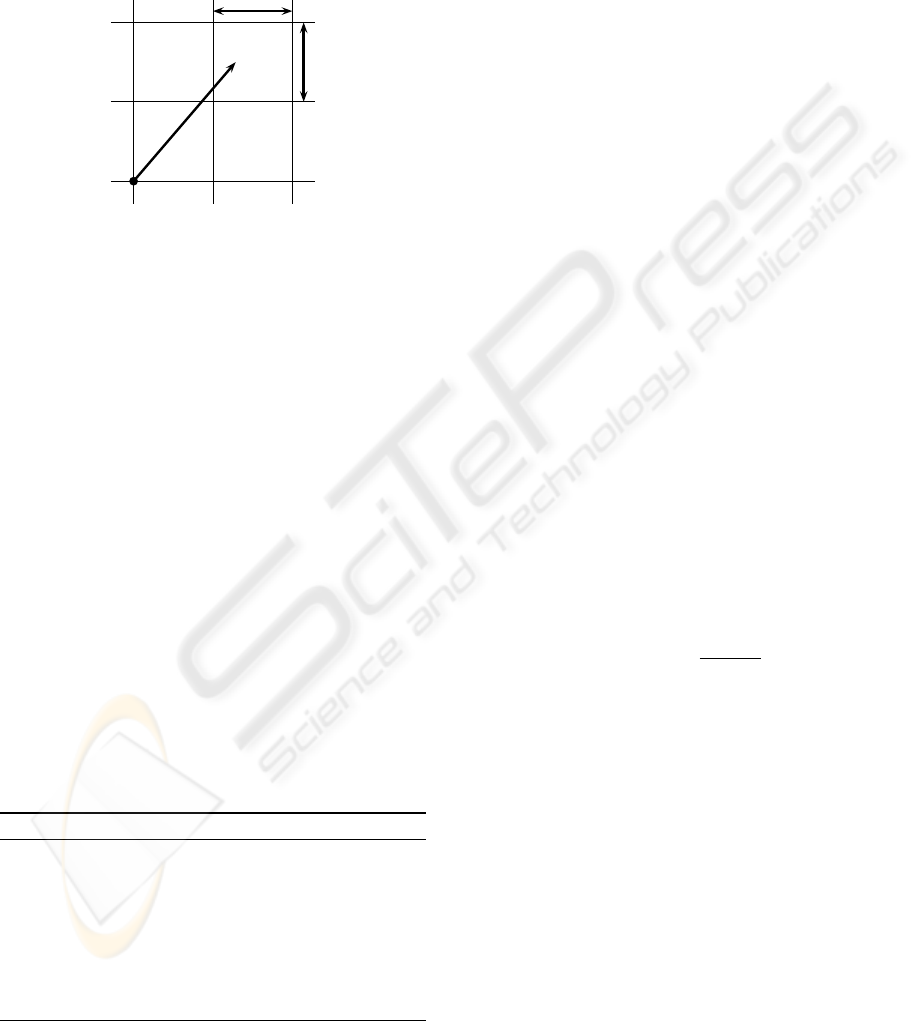
A straightforward way to adapt Algorithm 1 in this

continuous context is ﬁrst to discretize time and space

and then to ﬁnd an equivalent of the Bellman equation

(2). Let us ﬁx a time step ∆t and a regular grid X

of resolution ǫ covering X . We evaluate V

∗

on each

point of the grid and interpolate for any x in X outside

(see ﬁgure 1).

′

Figure 1: Simple grid of resolution ǫ. V

is known at the

grid points, e.g. at x, whereas V

′

) has to be interpolated

In order to get a transition function, one can classi-

cally perform an Euler integration of (4):

→ x

′

⇔ x

′

= x + ∆x (5)

where ∆x = f (x, u)∆t

Moreover we can write :

) =

∆t

−s

c(x(t), u(t))dt

∞

∆t

−s

c(x(t), u(t))dt

≃ c(x(0), u(0))∆t + e

−s

∆t

(x(0) + ∆x)

≃ c(x

, u

)∆t + γV

+ ∆x) (6)

Where we note e

−s

∆t

= γ then V

∗

satisﬁes

∗

(x) ≃ min

u, x

→x

′

c(x, u)∆t + γV

∗

′

) (7)

which provides a decent equivalent of the discrete

Bellman equation. From here, nothing prevents us

from applying Algorithm 1 using (7) as a ﬁx point

iteration. The complete algorithm is given below.

Algorithm 2 Continuous Value Iteration

1: Init V

, i ← 0

2: repeat

3: for all x ∈ X do

4: V

i+1

(x) ← min

u, x

→x

′

c(x, u)∆t + γV

′

)

5: end for

6: i ← i + 1

7: until V

has converged

Again, Algorithm 2 is guaranteed to converge for

the same reasons as Algorithm 1 does, and, moreover,

in (Munos, 2000) it is proven that under certain reg-

ularity conditions, as ǫ and ∆t tend toward zero, V

tends toward the exact optimal VF of the continuous

problem.

2.3 Discussion

Limitations As presented above, the adaptation of

discrete value iteration algorithm to the continuous

case may seem simple. Unfortunately, in practice it

may fail for several reasons: ﬁrst, as it is a direct

application of DP, it has the limitation that Bellman

called originally the curse of dimensionality (Bell-

man, 1957) which expresses the fact that complexity

of these algorithms is exponential in the dimension of

the system. This makes them impractical for prob-

lems in high dimensions. Another limitation of Algo-

rithm 2 that is more speciﬁc to the continuous case is

the simplicity of the underlying numerical methods.

Explicit Euler integration used in (5) is the simplest

method to solve a differential equations and is known

to have severe limitations. In particular, it is of or-

der one and is sensitive to stiffness. Also, in (6), the

rectangle method is used to approximate integral on

interval [0, ∆t] which is also a method of order one.

A lot can be done to beneﬁt from more clever nu-

merical schemes to solve (4) or to better approxi-

mate the integral in (6) using more advanced meth-

ods of numerical analysis. For instance, backward

Euler integration is preferable to explicit Euler inte-

gration (Doya, 2000) and a cost-less trick to improve

approximation (6) consists in, instead of considering

that e

−s

c(x, u) is constant on [0, ∆t], only consid-

ering that c(x, u) is constant and integrating formally

the exponential, which gives, if γ = e

−s

∆t

∗

(x) ≃ min

u, x

→x

′

c(x, u)

(1 − γ)

+ γV

∗

′

) (8)

which is a more precise continuous equivalent of the

discrete Bellman equation than (7) that can be used in

Algorithm 2 (Coulom, 2002).

Function approximators The major reason for the

curse of dimensionality is the discretization of the

state space into a simple grid, an object whose size

grows exponentially with the number of dimensions.

Among classical alternative solutions are variable

resolution discretization (Munos and Moore, 1999),

sparse coarse coding (Sutton, 1996), or neural net-

works (Coulom, 2002), (Tesauro, 1995). It is worth

recalling that all these techniques, including simple

grids, approximate a function deﬁned over (a bounded

subset of) R

using a ﬁnite number of parameters

{ω

, i ∈ N}. In the case of simple grids, these

parameters are associated to the exponentially many

ON TEMPORAL DIFFERENCE ALGORITHMS FOR CONTINUOUS SYSTEMS

grid points. In the case of neural networks, the pa-

rameters are the weights of the “neurons” in the net-

work, whose number is dimension independent. Al-

though methods using sophisticated function approx-

imators like neural networks proved to be potentially

very powerful in some practical cases, such as for

swimmers in (Coulom, 2002), they offer in general no

guarantee of convergence or optimality. In fact, func-

tion approximators are double-edged swords. On one

hand, they provide generalization, that is, while the

VF is updated at a point x, it is also updated in some

neighborhood of x, or more precisely in all points af-

fected by the change of the parameters of the approx-

imator; the bad side is interference which is in fact an

excessive generalization, e.g. if an update in x affects

the VF in y in such a way that it destroys the beneﬁts

of a previous update in y. Understanding and control-

ling the effects of generalization, in particular in the

case of non linear function approximators, is a very

deep and complicated numerical analysis problem.

Hamilton-Jacobi-Bellman (HJB) Equation Here

we present the connection with the HJB Equation.

In fact, (7) and (8) can be seen as ﬁnite differences

schemes approximating the HJB equation, that we can

retrieve from those equations by dividing each term

by ∆t and making ∆t going to zero, which leads to

min

u∈U



c(x, u) +

∂V

∗

∂x

· f (x, u) − s

∗

(x)



= 0 (9)

From this deﬁnition of the HJB equation, we deﬁne

the Hamiltonian:

H(x) = min

u∈U

c(x, u) +

∂V

∂x

· f(x, u) − s

(x)

(10)

Algorithms for computing V

∗

thus often try to mini-

mize H in order to ﬁnd a solution to (9). The problem

is that there might be an inﬁnite number of general-

ized solutions of (9) i.e. functions that satisfy H(x) =

0 almost everywhere, while being very far from the

true value function V

∗

(Munos, 2000). Thus, if no

guarantee is given by the algorithm other than the

minimization of H(x), then no one can tell whether

the computed solution is optimal or even near to the

optimal VF.

(Munos, 2000) uses the theory of viscosity solutions

to prove that Algorithm 2 actually converges toward

the true value function but this result is limited to the

case of grids.

3 TEMPORAL DIFFERENCE

ALGORITHMS

DP algorithms presented so far compute the next es-

timation V

i+1

(x) based on V

(x) and V

′

) where

′

is in the spatial neighborhood of x. The slightly

different point of view taken by temporal difference

(TD) algorithms is that instead of considering that

′

is the neighbor in space of x they consider it as

its neighbor in time along a trajectory. This way,

with the same algorithm, V

i+1

(x) would be updated

from V

(x(0)) and V

(x(∆t)), where x = x(0) and

′

= x(∆t) are then viewed in the context of a whole

trajectory (x(t))

t>0

. Then, pursuing in this spirit, it is

clear that if V

(x(∆t)) holds interesting information

for the update of V

(x(0)), then it is also the case for

(x(t)) for all t > 0. Henceforth, TD algorithms

update their current approximation of the VF thanks

to data extracted from complete trajectories.

3.1 General Framework

In section 2, we discussed the fact that DP algo-

rithms were bound to different issues and problemat-

ics: function approximation, numerical analysis etc.

This was the case for value iteration algorithms and

their adaptation to continuous time and space, and this

is also the case for TD algorithms. In this subsection,

we propose a general, high level framework common

to most of TD algorithms that allow us to separate

those different issues, assuming that some are solved

and focusing on the others. This high-level frame-

work is represented by Algorithm 3.

Algorithm 3 Generic TD algorithm

1: Init V

, i ← 0

2: repeat

3: Choose x

∈ X

4: Compute (x(t))

t∈[0,T ]

using u(·), starting

from x

5: Compute update trace e(·) from x(·) and u(·)

6: for all t ∈ R

7: V

i+1

(x(t)) ← V

(x(t)) + e(t)

8: end for

9: i ← i + 1

10: until Stopping condition is true

To implement an instance of this generic algorithm,

we need the non-trivial following elements:

• A simulator that can generate a trajectory of dura-

tion T > 0 (x(t)))

t∈[0,T ]

given an initial state x

and an input function u.

• A function approximator to be used to represent

any function V from X to R

and allowing us to

simply write V (x) for any x in X e.g. lines 7. A

question arising here is, as already discussed in pre-

vious sections, whether to use simple grids, linear

function approximators, or non linear function ap-

proximators such as neural networks etc.

ICINCO 2005 - INTELLIGENT CONTROL SYSTEMS AND OPTIMIZATION

• An update function which, given a function V , a

state x and a quantity e, alters V

into V

i+1

so that

i+1

(x) is equal to or near V

(x) + e, which is

written line 7 as an assignment statement. When

parametrized function approximators are used, up-

dating can be done e.g. by gradient descent on the

parameters (Doya, 2000).

• A policy, or controller, which returns a control in-

put at each time t, needed by the simulator to com-

pute trajectories. In the case of optimistic policy it-

eration (Tsitsiklis, 2002), u is the feedback control

obtained from V

using the arg min of left hand

side of (10). It is said to be optimistic because if V

is the optimal VF, then this gives an optimal control

input.

• An update trace generator used to extract infor-

mation from the computed trajectory x(·) and to

store it into the update trace e(.) (line 5). In the

ﬁeld of RL, e(.) is classically called the eligibility

trace (Sutton and Barto, 1998).

Variants of TD algorithms differ in the way this last

point is implemented, as discussed in the following

sections.

3.2 Continuous TD(λ)

3.2.1 Formal algorithm

The objective of TD algorithms is to build an im-

proved estimation of the VF based on the data of com-

puted trajectories. The main additional information

provided by a trajectory x(·) is the values of the cost

function along its course. If we combine these values

with the current estimation V

, we can then build a

new estimation for a given horizon τ > 0, which is:

) =

−s

c(x, u)dt + e

−s

(x(τ)) (11)

In other words, the estimation

) relies on a por-

tion of the trajectory of duration τ and on the old es-

timation V

(x(τ)) at the end of this portion. We re-

mark that if V

is already the optimal value function

∗

, then

= V

∗

for all τ > 0 and this equality is,

in fact, a generalization of the Bellman equation.

A question to answer is then, how to choose horizon

τ? In the case of TD(λ), the algorithm constructs

a new estimation

which is a combination of the

) for all τ > 0. In our continuous framework,

we deﬁne for s

> 0:

) =

∞

−s

)dτ (12)

Several remarks about this deﬁnition are:

• Equation (12) means that

is constructed from all

, τ > 0, each of them contributing with an expo-

nentially decreasing amplitude represented by the

term e

−s

. In other words, the further

looks

into the trajectory, the less it contributes to

• This deﬁnition is sound in the sense that it can be

seen as a convex combination of

, τ > 0. In

effect, it is true that

∞

−s

dτ = 1. Thus, if

each

is a sound estimation of V

∗

, then

is a

sound estimation of V

∗

• This deﬁnition is consistent with the original deﬁn-

ition of TD(λ) algorithm (Sutton and Barto, 1998).

In fact, by choosing a ﬁxed time step ∆τ , assum-

ing that

is constant on [τ, τ + ∆τ ] and summing

−s

on this interval, we get:

) ≃ (1 − λ)

∞

k=0

k∆τ

) (13)

where λ = e

−s

∆τ

which is the usual discrete TD(λ) estimation built

upon the k-step TD estimation (Tsitsiklis, 2002)

k∆τ

) =

k∆τ

−s

c(x, u)dt + e

−s

(x(k∆τ ))

≃

k−1

j=0

c(x(j∆τ ), u(j∆τ))+

−s

k∆τ

(x(k∆τ ))

k−1

j=0

c(x

, u

) + γ

) (14)

where γ = e

−s

∆τ

3.2.2 Implementation

In practice, we can only compute trajectories with a

ﬁnite duration T . As a consequence,

can only be

computed for τ ≤ T . In this context, (12) is replaced

) =

−s

)dτ + e

−s

)

≃ (1 − λ)

N−1

k=0

k∆τ

) + λ

)

where T = N ∆τ (15)

Combining (15) and (14), one can show that:

) −

) ≃

j=0

(16)

where

= c(x

, u

) + γV

j+1

) − V

) (17)

is what is usually referred to as the temporal differ-

ence error (Tsitsiklis, 2002). This expression pro-

vides an easy implementation given in Algorithm 4

ON TEMPORAL DIFFERENCE ALGORITHMS FOR CONTINUOUS SYSTEMS

which reﬁnes line 5 of Algorithm 3. There, we as-

sume that the trajectory has already been computed

with a ﬁxed time step ∆t = ∆τ, that is at times

= j∆t, 0 ≤ j ≤ N + 1.

Algorithm 4 TD(λ): Update traces

1: for j = 0 to N do

2: δ

← c(x

, u

) + γV

j+1

) − V

)

3: end for

4: e(t

) ← δ

5: for k = 1 to N do

6: e(t

N−k

) ← e(t

) + (λγ)e(t

N−k+1

)

7: end for

Note that the computation complexity of the update

trace is in O(N ) where N + 2 is the number of com-

puted points in the trajectory x. Thus the overall com-

plexity of the algorithms depends only on the num-

ber of trajectories to be computed in order to obtain a

good approximation of V

∗

3.2.3 Qualitative interpretation of TD(λ)

In the previous sections, we started by presenting

TD(λ) as an algorithm that compute a new estima-

tion of the VF using a trajectory and older estima-

tions. This allowed us to provide a continuous for-

mulation of this algorithm and an intuition of why

it should converge towards the true VF. Then, using

a ﬁxed time step and numerical approximations for

implementation purposes, we derived equation (16)

and Algorithm (4). These provide another intuition of

how this algorithm behaves.

The TD error δ

(17) can be seen as a local error in

x(t

) (in fact, it is an order one approximation of the

Hamiltonian H(x(t

))). Thus, (16) means that the lo-

cal error in x(t

) affects the global error estimated by

TD(λ) in x(t

) with a shortness factor equal to (γλ)

The values of λ ranges from 0 to 1 (in the continuous

formulation, s

ranges from 0 to ∞). When λ = 0,

then only local errors are considered, as in value iter-

ation algorithms. When λ = 1 then errors along the

trajectory are fully reported to x

. Intermediate val-

ues of λ are known to provide better results than these

extreme values. But how to choose the best value for

λ remains an open question in the general case. Our

intuition, backed by experiments, tends to show that

higher values of λ often produce larger updates, re-

sulting in a faster convergence, at least at the begin-

ning of the process, but also often return a coarser

approximation of the VF, when it does not simply di-

verge. On the other hand, smaller values of λ result in

a slower convergence but toward a more precise ap-

proximation. In the next section, we use this intuition

to design a variant of TD(λ) that combines the quali-

ties of high and low values of λ.

3.3 TD(∅)

3.3.1 Idea

The new TD algorithm that we propose is based on

the intuition about local and global updates presented

in the previous section. Global updates are those per-

formed by T D(1) whereas local updates are those

used by T D(0). The idea is that global updates

should only be used if they are “relevant”. In other

cases, local updates should be performed. To de-

cide whether the global update is “relevant” or not,

we use a monotonicity argument: from a trajectory

x(·), we compute an over-approximation

V (x(t)) of

∗

(x(t)), along with the TD error δ(x(t)). Then,

V (x(t)) is less than the current estimation of the

value function V

(x(t)), it is chosen as a new estima-

tion to be used for the next update. In the other case,

(x(t)) + δ(x(t)) is used instead.

Let us ﬁrst remark that since c is bounded and s

> 0,

then V

∗

(x) ≤ V

max

, ∀x ∈ X , where

max

∞

−s

¯c dt =

¯c

(18)

This upper bound of V

∗

represents the cost-to-go of

an hypothetic forever worse trajectory, that is, a tra-

jectory for which at every moment, the pair state in-

put (x, u) has the worse cost ¯c. Thus, V

max

could be

chosen as a trivial over-approximation of V

∗

(x(t)).

In this case, our algorithm would be equivalent to

T D(0). But if we assume that we compute a tra-

jectory x(·) on the interval [0, T ], then a better over-

approximation can be obtained:

V (x

) =

−s

c(x, u)dt + e

−s

max

(19)

It is easy to see that (19) is indeed an over-

approximation of V

∗

(x(0)): it represents the cost of a

trajectory that would begin as the computed trajectory

x(·) on [0, T ], which is at best optimal on this ﬁnite

interval, and then from T to ∞ it behaves as the ever

worse trajectory. Thus,

V (x

) ≥ V

∗

3.3.2 Continuous Implementation of TD(∅)

In section 3.2.2 we ﬁxed a time step ∆t and gave a nu-

merical scheme to compute estimation

. This was

useful in particular to make the connection with dis-

crete TD(λ). In this section, we give a continuous

implementation of TD(∅) by showing that the compu-

tation of

V can be coupled with that of the trajectory

x(·) in the solving of a unique dynamical system.

Let x

(t) =

−s

c(x, u)dr. Then,

V (x

) = x

(T ) + e

−s

(T )

max

ICINCO 2005 - INTELLIGENT CONTROL SYSTEMS AND OPTIMIZATION

and more generally, for all t ∈ [0, T ],

V (x(t)) = e

(T ) − x

(t)) + e

−s

(T −t)

max

Where x

can be computed together with x by solv-

ing the problem:

(

˙x(t) = f(x(t), u(t))

˙x

(t) = e

−s

c(x(t), u(t))

x(0) = x

, x

(0) = 0

(20)

From there, we can give Algorithm 5.

Algorithm 5 TD(∅)

1: Init V

with V

max

, i ← 0

2: repeat

3: Choose x

∈ X

4: Compute (x(t))

t∈[0,T ]

and (x

(t))

t∈[0,T ]

solving (20)

5: Compute

V (x(·)) and δ(x(·))

6: for all t ∈ [0, T ] do

7: V

i+1

(x(t)) ← min(

V (x(t)), V

(x(t)) +

δ(x(t)))

8: end for

9: until Stopping condition is true

Several remarks are worth mentionning:

• Initializing V

to V

max

imposes a certain

monotonicity with respect to i. This monotonic-

ity is not strict since when local updates are made,

nothing prevents δ(x(t)) from being positive, but

during the ﬁrst trajectories at least, as long as they

pass through unexplored states,

will be auto-

matically better than the pessimistic initial value.

Note also that if V

∗

is known at some special states

(e.g. at stationary points), convergence can be fas-

tened by initializing V

to these values.

• Computing x and x

(and hence

V ) together in the

same ordinary differential equation (ODE) facili-

tates the use of variable time step size integration,

the choice of which can be left to a specialized efﬁ-

cient ODE solver, and thus permits a better control

of the numerical error at this level.

4 EXPERIMENTAL RESULTS

To compare the performances of TD(∅) with TD(λ)

for various values of λ, we implemented and applied

Algorithms 4 and 5 to deterministic, continuous ver-

sions of two classical problems in the ﬁeld of RL:

The continuous walker: a one dimensional problem

in which a robot must exit the zone [−1, 1] as

quickly as possible. The system equations are

given by

˙x =

(

u if −1 < x < 1

min(0, u) if x = 1

max(0, u) if x = −1

(21)

The input u represents the speed of the walker in

either direction. It is bounded in absolute value by

1. Thus, in the context of optimal control, we can

restrict to a binary decision problem where u = 1

or u = −1. The cost function is:

c(x) =



1 if −1 < x < 1

0 if x = −1 or x = −1

(22)

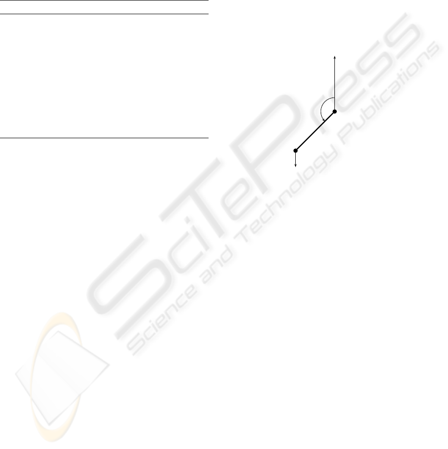
The swing-up of a pendulum with limited torque.

The goal is to drive a pendulum to the vertical posi-

tion. The dynamics of the system are described by

a second order non linear differential equation:

θ = −µ

θ + g sin θ + u (23)

−10 <

θ < 10, −3 < u < 3

Figure 2: Pendulum

The cost function is c(θ) = (1 − cos(θ)). It is thus

minimal, equal to 0 when the pendulum is up (θ =

0) and maximal, equal to 2, when the pendulum is

down. The variable µ is a friction parameter and g

the gravitational constant.

For both of these problems, we used regular grids and

linear interpolation to represent values of V

. We call

a sweep a set of trajectories for which the set of ini-

tial states cover all points of the grid. For both prob-

lems, we then applied TD(λ) and TD(∅) to such set of

trajectories and after each sweep, we measured the 2-

norm of the Hamiltonian error (noted kδk

) over the

state space. This allowed to observe the evolution of

this error depending on the number of sweeps of the

state space performed.

The results are given in ﬁgure 3 and 4. An interesting

thing to observe is that for the simple problem of the

walker, the value of λ that worked best in our exper-

iments was 0, whereas for the pendulum, this value

was more around 0.7. Not surprisingly, in the ﬁrst

case, we see that the error curve of TD(∅) closely fol-

lows that of T D(0), even performing slightly better.

For the second problem, TD(∅) seems to perform bet-

ter than TD(λ) for any value of λ. This leads to the

very encouraging observation that TD(∅) seems to be-

have at least as well as TD(λ) for the best value of λ,

independently of this value and of the problem. Of

course, more experiments are needed to validate this

conclusion.

ON TEMPORAL DIFFERENCE ALGORITHMS FOR CONTINUOUS SYSTEMS

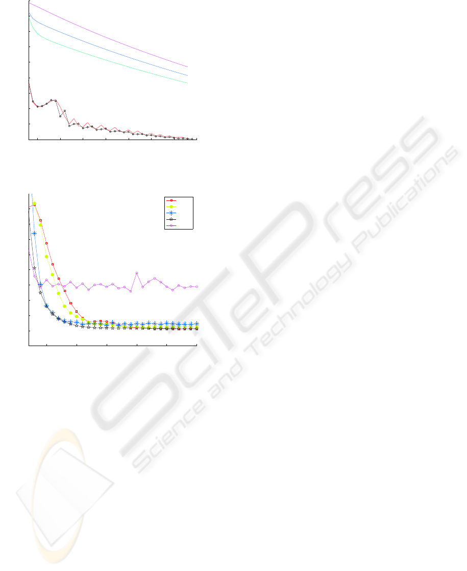
5 10 15 20 25 30 35 40

0.005

0.01

0.015

0.02

0.025

0.03

0.035

0.04

0.045

# of Sweeps

||δ||

Hamiltonian error

λ=1

λ=0.5

λ=0.75

λ=0

TD()

Figure 3: Hamiltonian error for walker

5 10 15 20 25 30

0.01

0.02

0.03

0.04

0.05

0.06

0.07

0.08

0.09

# of sweeps

||δ||

Hamiltonian error

λ=0

λ=0.25

λ=0.75

TD()

λ=1

Figure 4: Hamiltonian error for pendul

5 CONCLUSIONS

We have presented a framework for the design of tem-

poral differences algorithms for optimal control prob-

lems in continuous time and space. This framework

is attractive as it clearly separates different issues re-

lated to the use of such algorithms, namely:

1. How to choose and compute trajectories - which

initial state, and which choice of u - in order to

ensure that the VF will be accurately and quickly

computed in the interesting part of the state space?

2. How to represent the VF efﬁciently in order to

break the curse of dimensionality?

3. How to update the VF based on simulated trajecto-

ries?

After describing the context of DP and our frame-

work, we focused on question 3 and presented a con-

tinuous version of TD(λ) which was shown to be con-

sistent after appropriate discretization with the origi-

nal discrete version of the algorithm. We then dis-

cussed its efﬁciency with respect to the parameter λ,

and presented a variant, TD(∅), that we found to be

experimentally as efﬁcient as TD(λ) for the best val-

ues of λ. Future work will include improvement of

this algorithm and its application to higher dimen-

sional problems, and consequently an investigation of

the above mentioned Questions 1 and 2,a necessary

step toward scalability.

ACKNOWLEDGMENTS

I am grateful to Oded Maler, Thao Dang and Eugene

Asarin for helpful discussions, comments and sugges-

tions. This work was partially supported by the Euro-

pean Community projects IST-2001-33520 CC (Con-

trol and Computation).

REFERENCES

Bellman, R. (1957). Dynamic Programming. Princeton

University Press, Princeton, New Jersey.

Coulom, R. (2002). Reinforcement Learning Using Neural

Networks, with Applications to Motor Control. PhD

thesis, Institut National Polytechnique de Grenoble.

Doya, K. (1996). Temporal difference learning in continu-

ous time and space. In Touretzky, D. S., Mozer, M. C.,

and Hasselmo, M. E., editors, Advances in Neural In-

formation Processing Systems, volume 8, pages 1073–

1079. The MIT Press.

Doya, K. (2000). Reinforcement learning in continuous

time and space. Neural Computation, 12(1):219–245.

Munos, R. (2000). A study of reinforcement learning in the

continuous case by the means of viscosity solutions.

Machine Learning, 40(3):265–299.

Munos, R. and Moore, A. (1999). Variable resolution dis-

cretization for high-accuracy solutions of optimal con-

trol problems. In International Joint Conference on

Artiﬁcial Intelligence.

Rantzer, A. (2005). On relaxed dynamic programming in

switching systems. IEE Proceedings special issue on

Hybrid Systems. Invited paper, to appear.

Sutton, R. S. (1996). Generalization in reinforcement learn-

ing: Successful examples using sparse coarse coding.

In Advances in Neural Information Processing Sys-

tems 8, pages 1038–1044. MIT Press.

Sutton, R. S. and Barto, A. G. (1998). Reinforcement Learn-

ing: An Introduction. MIT Press, Cambridge, MA.

Tesauro, G. (1995). Temporal difference learning and TD-

Gammon. Communications of the ACM, 38(3):58–68.

Tsitsiklis, J. N. (2002). On the convergence of optimistic

policy iteration. Journal of Machine Learning Re-

search, 3:59–72.

ICINCO 2005 - INTELLIGENT CONTROL SYSTEMS AND OPTIMIZATION