MULTI-OBJECTIVE PREDICTIVE CONTROL: APPLICATION
FOR AN UNCERTAIN PROCESS
Anes Bedoui
Laboratoire d’Analyse et Commande des Systèmes (ACS), ENIT, Tunisie.
Faouzi Bouani, Mekki Ksouri
Institut National des Sciences Appliquées et de Technologie, Tunis, Tunisie
Keywords: Predictive control; multi objective optimization; laboratory process; weighting functions method.
Abstract: This paper deals with the application of the Multi Objective Generalized Predictive Control (MOGPC) to
level control in a laboratory process. The major characteristic of the considered plant is that the manual
draining vane can take many positions causing changes in plant dynamics and strong disturbances in the
process. The controller is based on a set of Controlled Auto Regressive Integrated Moving Average
(CARIMA) model. The Recursive Least Squares (RLS) algorithm is used to estimate each model
parameters. The control law is obtained by minimizing a multi objective optimization problem. The
weighting sum approach is considered to formulate the control problem as a single criterion optimisation
one. The real time control system implementation confirms the opportunity of using the MOGPC scheme to
an uncertainty system.
1 INTRODUCTION
The Generalized Predictive Control (GPC) principle
consists in calculating the control input by the
minimization of a cost function over a future time
horizon under certain process constraints (Clarke et
al. 1987). Since the constraints on the input and the
output signals can be explicitly taken in account by
the GPC, this approach of control has attracted the
attention of many control researchers and industrials
(Boucher and Dumur 1996, Ben Abdennour et al.
2001).
Dynamics of industrial plants are usually not
completely known and are subject to change from
time to time. The complexity of industrial process
makes difficult their representation by only one
model. Consequently, the strategy which consists to
characterize the system with several models, every
model possessed its own validity domain, has been
developed (Brian and Bequette 2001). The strategy
of multi model control suffers from the difficulty of
determination model’s validity especially in noisy
systems. Another technique can be used to handle
nonlinear systems is the robust control design.
Robust controllers explicitly consider the
parametric variation in the process model for
calculating the control law (Gutierrez and Camacho
1995, Oliveira et al. 2000, Brdys and Chang, 2002).
The introduction of the uncertainty parameters leads
to the resolution of a min-max optimisation problem
which is hard to solve (Ramirez et al. 2002).
This paper presents the application of multi
objective predictive controller to an uncertain plant.
The major characteristic of the considered plant is
that the manual draining vane can take many
positions causing changes in plant dynamics and
strong disturbances in the process. Each operating
region can be modelled with a CARIMA model. The
Recursive Least Squares (RLS) algorithm is used to
estimate the model parameters. The control law is
obtained by minimizing a multi objective
optimization problem. The weighting sum approach
is considered to formulate the control problem as a
single criterion optimisation one.
This paper is organized as follows. Section 2
presents the description of the process. Section 3 is
reserved to the multi criteria generalized predictive
control based on a set of CARIMA model; the use of
the weighting functions method is also described.
233
Bedoui A., Bouani F. and Ksouri M. (2005).
MULTI-OBJECTIVE PREDICTIVE CONTROL: APPLICATION FOR AN UNCERTAIN PROCESS.
In Proceedings of the Second International Conference on Informatics in Control, Automation and Robotics - Signal Processing, Systems Modeling and
Control, pages 233-238
DOI: 10.5220/0001181602330238
Copyright
c
 SciTePress

Section 4 gives the results obtained in real time from
the water level regulation. The final section of the
paper presents the conclusion.
2 PROCESS DESCRIPTION
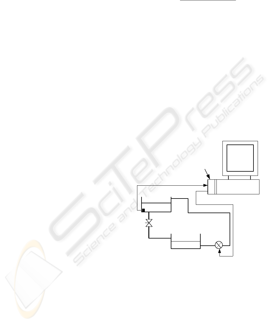
The process is schematically depicted in figure 1.
The main goal is to control in closed loop the level
in tank 1 by adjusting the liquid flow rate with the
electric actuator pump. The sampling time period is
fixed to 4s. While exploiting different step
responses, we give in figure 2 the steady state
characteristic. Then, the relation between the level
and the flow rate is non linear. It’s well known that
the capacity dominated process can be described by
a first order linear differential equation about a
desired operating level (William et al. 2000).
With the considered process, the manual
draining vane can take different positions then the
system can be modeled with an uncertainty first
order model. In order to identify the model
parameters, we have recorded two files of measures
giving the evolution of the water level for a shape of
crenel control. The obtained data, for the first and
the second positions of the draining vane, are
respectively represented in Figure 3 and Figure 4.
The presence of a numeric model is a necessary
condition for the development of the predictive
control, since it permits to calculate the predicted
output on a finished horizon. Consider the single
input single output process, which may be described
by the CARIMA model as follows (Clarke et al.
1987):
)()()()(
11
kuqBkyqA ∆=∆
−−
, (1)
where y(k) is the output signal and u(k) is the input
signal
. The term
1
1
−
−=∆ q
corresponds to an
integral action which permits the annulment of the
permanent regime error.
)(
1−
qA
and
)(
1−
qB
are
polynomials of degrees n
a
and n
b
in backward shift
operator q
-1
:
a
n
na
qaqaqA
−
−−
+++= ...1)(
1
1
1
, (2)
b
n
nb
qbqbqB
−
−−
++= ...)(
1
1
1
. (3)
For each operating region, a local CARIMA model
is determined. The model parameters are identified,
off-line, by using the (RLS) algorithm:
)()1(
ˆ
)()( kkkyke
T
φθ −−=
(4)
)()()()1(
ˆ
)(
ˆ
kekkPkk φθθ +−=
(5)
)()1()(1
)1()()()1(
)1()(
kkPk
kPkkkP
kPkP
T
T
φφ
φφ
−+
−−
−−=
(6)
where e(k) is the prediction error;
[]
T
nbna
bbaak ......)(
11
= θ is the parameter vector;
[]
T
nbkukunakykyk )(...)1()(...)1()( −−−−−−= φ
is the observation vector and P(k) is the covariance
matrix.
The input output data, considered in this work,
belong to two different working points. These data
given by figures 3 and 4 lead, respectively, to the
following models:
[]
T
k 0372.09864.0)(
1
−= θ and
[]
T
k 0301.09803.0)(
2
−= θ (7)
Personal computer
pump
Tank 2
Tank 1
Tank Level
Data
acquisition
device
Manual draining
vane
Figure 1: Laboratory process of level control
ICINCO 2005 - SIGNAL PROCESSING, SYSTEMS MODELING AND CONTROL
234

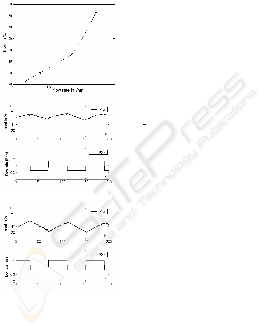
Figure 2: Non linear steady state characteristic
Figure 3: The water level y(k) and the flow rate u(k) (first
position of the draining vane).
Figure 4: The water level y(k) and the flow rate u(k)
(second position of the draining vane)
3 CONTROL AND DESIGN
For systems that present several modes of working,
different models can be built which are specific to
every mode of particular working of the system. We
consider the set of models:
{} )(,...),(
1
kkM
n
θθ =
(8)
where n is the number of possible models. A
multicriteria optimisation problem can be formulated
as follows:
()
n
U
JJ ...,,min
1
∆
(9)
where J
i
is formulated by using the model )(k
i
θ .
3.1 Single criterion GPC
The objective of the generalized predictive control
results in the minimization of the criterion under the
following analytic relation (Clarke et al. 1987):
()()
()
()()
⎟
⎟
⎠
⎞
⎜
⎜
⎝
⎛
∑∑
+∆++−+=
=
−
=
2
1
1
0
2
2
/
ˆ
2
1
N
j
u
N
j
c
jkujkykjkyJ λ
(10)
where N
2
is the prediction horizon, N
u
is the control
horizon,
λ
is the control increments weighting
factor, )(ky
c
is the set point, () kjky /
ˆ
+ ,
],1[
2
Nj ∈
, is the j step ahead predicted output and
)(ku
∆ is the control increment.
The minimization of the criterion requires the
computation of the predicted output over the
prediction horizon i.e.:
() kjky /
ˆ
+ ,
],1[
2
Nj ∈
. This
can be achieved by the model of the process. The j
step ahead predicted output is given by the following
relation (Clarke et al. 1987, Ben Abdennour et al.
2001).
)/()/()/(
ˆ
kjkykjkykjky
a
f
+++=+
(11)
where
)1()/( −+∆=+ jkuQkjky
j
f
and
() )(1)/( kyGkuRkjky
jja
+−∆=+
where Q
j
, R
j
and G
j
are polynomials solutions of
Diophantine equations.
On a prediction horizon N
2
and on a control horizon
N
u
, it is possible to transcribe equation (11) under
matrix shape:
a
UHYHUQY ∆++∆=
21
ˆ
(12)
where
Y
ˆ
is the vector of the predicted output,
U
∆
is
the vector of the present and the future control
increments. The vector
Y
is formed by the present
MULTI-OBJECTIVE PREDICTIVE CONTROL: APPLICATION FOR AN UNCERTAIN PROCESS
235

value and the old values of the output, the vector
a
U∆
is formed by the old increments of the control,
matrices
H
1
, H
2
and
Q
are formed, respectively, by
the coefficients of polynomials
j
G ,
j
R and
j
Q .
Based on these notations, we can write the criterion
J in the following matrix form
UUYYYYJ
T
c
T
c
∆∆+−−= λ ]
ˆ
[]
ˆ
[
(13)
where
Y
c
is the vector formed by the future set point
sequence.
The optimal solution is obtained while annulling the
gradient of
J in relation to the vector of the
increment control:
)(][
1
lc
T
N
T
YYQIQQU
u
−+=∆
−
λ (14)
where I
Nu
is a unity matrix of dimension (N
u
,N
u
) and
al
UHYHY ∆+=
21
.
The GPC is a receding control strategy, only the first
element of the vector
U
∆
is used to compute the
control to be applied to the process.
)1()1()( Ukuku ∆+−=
(15)
3.2 Multi objective GPC
The objectives are often conflicting or competing. A
powerful method for dealing with multiple
objectives is the Pareto optimality concept. Multi
objective problems usually have no unique solution,
but a set of non dominated solutions, known as the
Pareto optimal set (Xin et al. 2004). In the case of
non convex objectives, genetic algorithms are used
to solve the multi objective problems (Colette and
Siarry 2002, Silva and Fleming 2002, Andrès-Toro
et al. 2002). In this work, local models are linear,
consequently, the criterion J
i
is convex in the
controller parameters and it can be efficiently solved
by the weighting sum approach. The weighting
functions method transforms the multi criteria
problem to a single criterion one as follows (Colette
and Siarry 2002).
∑
=
=
n
i
ii
JwJ
1
(16)
where
∑
=
=
n
i
i
w
1
1 and 0≥
i
w . (17)
The weighting sum approach consists to take all
objectives in a single aggregating function. The
modification of the w
i
values that respect the
constraint (17), leads to the Pareto optimal set. Since
the optimization problem is convex, the solutions are
uniformly repatriated on the Pareto surface. In this
work, we have considered the optimal control, the
value from the Pareto set that gives the minimum of
the sum of all objectives.
The following algorithm is used to compute the
optimal sequence of control:
1- Take w
1
=0 and fix the step ∆ w
1
.
2- Choose w
i
, i=2,…,n that verify the relation
(17),
3- Compute
U
J
i
∆∂
∂
using (14) and
U
J
∆∂
∂
.
4- Compute the control sequence
)(kU∆
.
5- Increment
w
1
(w
1
=w
1
+ ∆ w
1
), if w
1
<1, return to
step 2.
6- Take
opt
U∆ that gives the minimum of the
sum of all criteria.
7- Compute the control law as follows:
)1()1()(
opt
Ukuku ∆+−=
In this algorithm, the size of the Pareto optimal set
depends on the choice of the step
∆ w
1
. In this work,
we have used
∆ w
1
=0.1, then at each sampling time,
we compute 10 solutions which form the Pareto set.
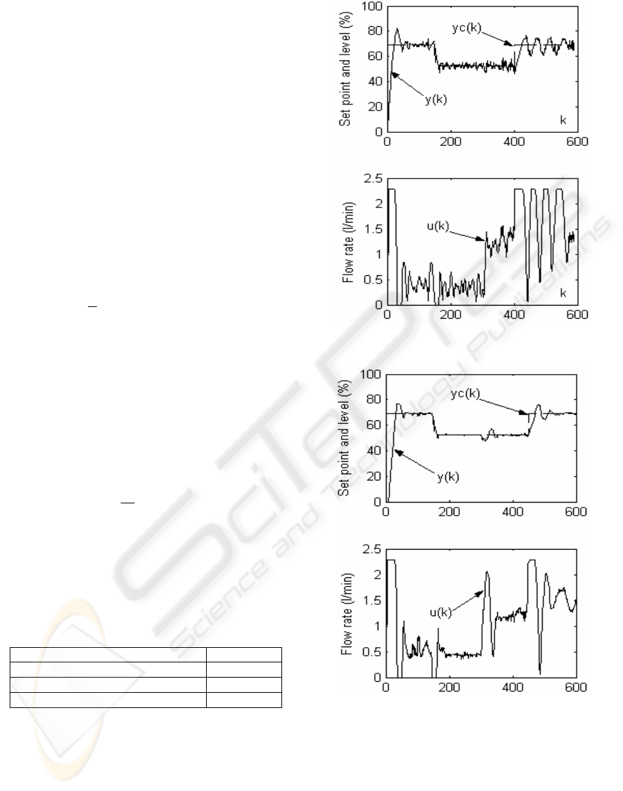
4 EXPERIMENT RESULTS
The multi objective predictive control scheme based
on the CARIMA model was applied to level control
in a laboratory process. In order to compare the
behavior of the standard GPC and the MOGPC in
presence of non-stationary process, we have fixed
the draining vane of the process described in section
2, in the first position during 300 sampling period
then we turn in the second position. The constraints
imposed on the input signal are as follows:
mnlku /3.2)(0 ≤≤ (18)
A discrete PID regulator can be given by the
following relation (Borne
et al. 1993):
)2()1()21(
)()1()1()(
−+−+−
+++−=
k
T
k
k
T
k
k
T
k
k
T
Kkuku
e
d
e
d
e
d
i
e
P
εε
ε
(19)
ICINCO 2005 - SIGNAL PROCESSING, SYSTEMS MODELING AND CONTROL
236

where K
p
is the proportional gain; k
i
is the integral
constant;
k
d
is the derivate constant; T
e
is the
sampling time period; and
ε(k) is the error between
the set point and the output signal. The PID
parameters are computed based on the step response
of the system and the Takahashi method (Borne
et
al.
1993).
The results obtained with the PID controller are
shown in Figure 5. The control signal presents many
fluctuations and the tracking error is not zero. In this
work, we have considered fixed PID controller
parameters. One can ameliorate the closed loop
performances by using an adaptive PID controller to
cope with the process dynamic changes. The results
obtained with the GPC are shown in Figure 6. In this
case, the controller is based on a nominal model
which is obtained by:
))()((
2
1
)(
21
kkk θθθ +=
(20)
It’s clear, from this figure, that the nominal model
assures good performances in closed loop. The
evolutions of the output/input and the set point
signals, in the case of the MOGPC, are given in
Figure 7. Obviously, we notice that performances in
terms of the tracking error and the variance of the
control signal are substantially ameliorated. Table 1
gives the variance of the control (
V) for the three
controllers.
()
∑
=
=
N
k
ku
N
V
1
2
)(
1
(21)
where N is the number of data measurement.
The variance obtained with the MOGPC is the
lower, because the control signal obtained with this
controller has few fluctuations compared to those
obtained with the GPC and the PID controllers.
Table 1: Variance of the control
Controller V
PID controller 1.6108
GPC (single criterion) 1.4546
GPC (multi objective strategy) 1.1248
Figure 5: PID controller (k
p
=0.5; k
i
=3; k
d
=0.1)
Figure 6: GPC (single quadratic criterion)
(N
2
= 7; N
u
= 1; 1=
λ
)
MULTI-OBJECTIVE PREDICTIVE CONTROL: APPLICATION FOR AN UNCERTAIN PROCESS
237

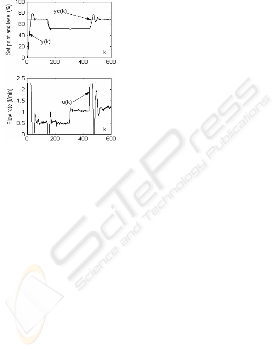
Figure 7: MOGPC (multi objective strategy)
(N
2
= 7; N
u
= 1; 1=
λ
)
5 CONCLUSIONS
This paper has presented the multi objective
predictive control. The process is characterized by a
set of CARIMA model. Since considered models are
linear, performance criteria are convex.
Consequently, the weighted sum approach is used to
compute the Pareto optimal set. An application of
the studied strategy to a nonlinear model plant has
been also presented.
REFERENCES
Andrès-Toro B., E. Besada-Portas, P. Fernandez-Blanco,
J. A. Lopez-Orozco, and J. M. Giron-Sierra, 2002,
“Multiobjective optimization of dynamic processes by
evolutionary methods”. Proc. 15
th
IFAC World
Congress, Barcelona, Spain.
Ben Abdennour R., P. Borne, M. Ksouri, F. M’sahli, 2001,
“Commande numérique et identification des procédés
industriels”. Editions TECHNIP, Paris.
Boucher P., and D. Dumur, 1996 “La commande
prédictive”. Editions TECHNIP, Paris.
Borne P., G. Dauphin Tangay, J. P. Richard, F. Rotella, I.
Zambe Hakis, 1993, "Analyse et régulation des
processus industriels", Tome 2. Régulation
numérique. Editions TECHNIP, Paris.
Brdys M. A. and T. Chang, 2002, “Robust model
predictive control under output constraints”. Proc. 15
th
IFAC Triennial World Congress, Barcelona/Spain.
Brian A., Vinay P., and B. W. Bequette, 2001, “A
comparison of fundamental Model based and Multiple
Model Predictive Control”. Proc. 40
th
IEEE
conference on Decision and Control, Orlando, Florida
USA, 4863-4868.
Clarke D. W., C. Mohtadi and P. S. Tuffs, 1987,
“Generalized predictive control”. Part I and Part II,
Automatica, 23, 2, 137- 160.
Colette. Y., Siarry. P., 2002, “Optimisation multiobjectif”.
Editions EYROLLES.
Gutierrez A. J. and E. F. Camacho, 1995, “Robust
adaptive control for processes with bounded
uncertainties”. Third European control conference.
Rome/Italy, 1295-1300.
Oliveira G. H. C., W. C. Amaral, G. Favier and G. A
Dumont, 2000, “Contrained robust predictive
controller for uncertain processes modelled by
orthonormal series function”. Automotica, 36, 563-
571.
Ramirez D. R., T. Alamo and E. F. Camacho, 2002,
“Efficient Implementation of constrained Min-Max
model Predictive Control with Bounded
Uncertainties”. Proc. IEEE Conference on Decision
and Control.
Silva V.V.R. and P.J. Fleming, 2002, “Control
configuration design using evolutionary computing”.
Proc. 15
th
IFAC World Congress, Barcelona, Spain.
William Y. S., P. M.Donald and R.Y. Brent, 2000, “A real
time approach to process control”. John Wiley &
Sons, Ltd.
Xin Q., Murti V. S., Petros G. V., and Mustafa K., 2004,
“Structured optimal and robust control with multiple
criteria: a convex solution”. IEEE Trans. on Automatic
Control, 49, 10, 1623-1640.
ICINCO 2005 - SIGNAL PROCESSING, SYSTEMS MODELING AND CONTROL
238