EXTENSION VERSUS BENDING FOR CONTINUUM ROBOTS

Robin McDonnell, George Grimes, and Ian D. Walker

Department of Electrical and Computer Engineering, Clemson University, Clemson 29634 USA

Carlos Carreras

Departamento de Ingenieria Electronica, E.T.S.I.T. Universidad Politecnica de Madrid, 28040 Madrid, Spain

Keywords: Robotics, Continuum, Manipulators, Intervals.

Abstract: In this paper, we analyze the capabilities of a n

ovel class of continuous-backbone (“continuum”) robots.

These robots are inspired by biological “trunks, and tentacles”. However, the capabilities of established

continuum robot designs, which feature controlled bending but not extension, fall short of those of their

biological counterparts. In this paper, we argue that the addition of controlled extension provides dual and

complementary functionality, and correspondingly enhanced performance, in continuum robots. We present

an interval-based analysis to show how the inclusion of controllable extension significantly enhances the

workspace and capabilities of continuum robots.

1 INTRODUCTION

Recent interest in expanding the capabilities of robot

manipulators has led to renewed interest in

continuous backbone “continuum” manipulators

(Robinson and Davies, 1999). The idea behind these

robots is to replace the “vertebrate” (serial chain of

rigid links) backbone of conventional manipulators

with a smooth, continuous, “invertebrate” backbone.

Continuum robots have the potential for

revolutionizing robot operations, by enabling new

applications (operation inside complex environments

such as collapsed buildings, rubble piles, etc.), and

via novel forms of manipulation (compliant and

whole arm manipulation, adaptive environmental

interaction).

The concept of continuum robots is not new

(Hi

rose, 1993). A number of designs have been

suggested, with a number of prototypes constructed

(Robinson and Davies, 1999). Most of these are

inspired by the biological examples of tongues

(Takanobu, Tandai and Miura, 2004), trunks

(Cieslak and Morecki, 1999), (Hannan and Walker,

2003), Tsukagoshi, Kitagawa and Segawa, 2001),

(Wilson, Li, Chen and George, 1993), and tentacles

(Aoki, Ochiai and Hirose, 2004), (Gravagne and

Walker, 2000), (Ohno and Hirose, 2001), Pritts and

Rahn, 2004), (Simaan, Taylor and Flint, 2004),

(Suzumori, Iikura and Tanaka, 1991). Several

designs have made their way to commercial products

(Buckingham and Graham, 2003), (Immega and

Antonelli, 1995).

In almost all of the above designs (with the

otable exceptions (Immega and Antonelli, 1995)

and (Pritts and Rahn, 2004)), movement of the

“backbone” is created by bending of the trunk at

discrete locations along its length. While this design

allows for the inclusion of redundant degrees of

freedom along the backbone, the degrees of freedom

available locally are less than in the biological

counterparts (Kier and Smith, 1985). In particular,

the ability to extend the “backbone”, present in

many invertebrate limbs (Kier and Smith, 1985) is

missing. This paper explores the functional gains

obtained by including this “missing” degree of

freedom in continuum robots.

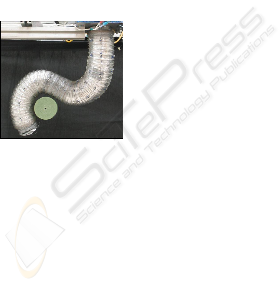
In recent work (Jones, McMahan and Walker,

04) we have developed a multi-section continuum

robot, Air-Octor, whose design features both

bending and extension (see figure 1). The design

extends that of (Immega and Antonelli, 1995) in that

the extension of each section can be independently

controlled (as opposed to only the total length

(Immega and Antonelli, 1995)). We are additionally

conducting applied research (McMahan, Jones,

Walker, Chitrakaran, Seshadri and Dawson, 2004)

258

McDonnell R., Grimes G., D. Walker I. and Carreras C. (2005).

EXTENSION VERSUS BENDING FOR CONTINUUM ROBOTS.

In Proceedings of the Second International Conference on Informatics in Control, Automation and Robotics - Robotics and Automation, pages 258-265

DOI: 10.5220/0001175502580265

 SciTePress

with the continuum robot hardware introduced in

(Pritts and Rahn, 2004), which also feature

controllable extension, as well as bending, in each

section. Our operational experience with these

robots (compared with our earlier series of

continuum arms which lacked extension (Gravagne

and Walker, 2000), (Hannan and Walker, 2003))

clearly indicates superior performance arising from

the additional degrees of freedom, even for arms

with comparable total degrees of freedom. This

paper analyzes and quantifies this effect, in terms of

the kinematic performance improvement.

Figure 1: Continuum Robot “Air-Octor.”

2 KINEMATICS

We wish to analyze and quantify how the inclusion

of controllable extension in continuum robots

increases the capability over previously developed

designs with only controllable bending. In particular,

from a task-based viewpoint, we are interested in

quantifying any workspace enhancement obtained

by adding extension. For this, we conduct a

comparative interval-based analysis of the forward

kinematics.

In our operational experience with Air-Octor

(Kier and Smith, 1985) and the “Oct-Arm” series of

continuum robots introduced in (Pritts and Rahn,

2004), we have found that the ability to extend the

lengths of sections is very useful. For example we

have found that active use of extension/contraction

can greatly assist the stability of whole arm

grasping, by effectively tightening and loosening the

grip. However, the effects of extension, and their

relationship to those bending, remain nonintuitive. A

tool which could be used to analyze these effects

would be valuable in practical motion planning. In

the following we introduce such a tool.

We restrict our analysis to planar movements,

for simplicity, and since this is sufficient to illustrate

the key advantages of adding extension.

The tip location for a two-section continuum

manipulator (for Air-Octor or Oct-Arm) when

operated in the plane is given by (Blessing and

Walker, 2004), (Jones and Walker, 2004):

111

21121 1

(1 / )[cos( ) 1]

(1/ )[cos( ( )) cos( )]

xk kl

kklkll kl

=−

++−−

111

21121 1

(1 / ) sin( )

(1/ )[sin( ( )) sin( )]

ykkl

kklkll kl

++−−

In the above,

represents the curvature of the

ith section, and l

stands for the section’s length, both

of which are controllable variables. From these

equations, it is possible to evaluate the significance

of including variable section lengths in addition to

variable curvatures. The primary objective of the

analysis is to assess the workspace enhancement of

the continuum robot. In addition, the probability of

reaching the locations within the workspace by

means of different robot configurations will also be

studied.

3 INTERVAL ANALYSIS

The method used for the analysis is based on multi-

interval computations which provide accurate

estimates for workspaces (i.e. 2D ranges) and have

been extended to support probability descriptions in

terms of probability density functions (PDFs).

Multi-interval computations are an extension of

interval analysis (Moore, 1979) that minimizes its

overestimation problem. This problem appears when

multiple instances of the inputs appear in the

equation or algorithm under study (i.e. there are

crossed data dependencies, as in the equations

above). This method parallels that in (Walker and

Carreras, 2003) where linear (straight line) links

were considered. It also refines the initial results in

(Blessing and Walker, 2004), where plain interval

arithmetic was used for the analysis of a different

continuum design, in which the bending location

could be mechanically adjusted off-line, but not

actively controlled.

Interval arithmetic allows fast and easy

computations on ranges of values by means of

computations on the intervals' endpoints (Moore,

1979). It is exact if there are no crossed data

EXTENSION VERSUS BENDING FOR CONTINUUM ROBOTS

259

dependencies, but otherwise it produces oversized

results. A classical example of this effect is known

as the cancellation problem: given an interval

I =

[

a,b], the computation I-I = [a-b,b-a] ≠ [0,0]. One

alternative to reduce overestimation is to use multi-

intervals: the original interval is divided into smaller

adjacent disjoint subintervals, the computation is

performed for each of them, and the individual

results are merged into a single interval result. In the

previous example, if I is represented by two

subintervals, [

a,(a+b)/2] and [(a+b)/2,b], the

merging of the individual results of the computation

I-I produces the interval [(

a-b)/2,(b-a)/2] ⊂ [a-b,b-

a], thus reducing overestimation. Greater reductions

are achieved if more subintervals are used.

Therefore, multi-intervals are a simple yet powerful

approach for function evaluation where increased

precision (i.e. using more subintervals) is directly

available at the cost of increased computation time.

The methodology to use multi-intervals has

been automated in an in-house framework called

Abaco, already used in (Walker and Carreras, 2003).

Abaco is based on the GNU Multiple Precision

Library GMP and includes all the tools used to carry

out this study. Abaco has also been successfully

used in other tasks related to reliability analysis and

digital electronic design, and is constantly upgraded

with new features and capabilities. Extensions to

handle probabilities (each interval can have a

probability, thus allowing the computation of output

PDFs from input PDFs) are also supported. The

significance analysis presented here has also

motivated specific extensions to handle

trigonometric functions and 2-dimensional outputs

(i.e. locations in the plane), in the computation and

graphics tools within the framework. In addition, the

tuning of the tools for each particular analysis has

been simplified to avoid test runs required in

previous versions of the tools. Using Abaco,

different multi-section robots can be quickly and

extensively analyzed by simply specifying their

kinematic equations.

The Abaco implementation is based on a

discretization of the numerical space that simplifies

the definition of two basic concepts: interval

adjacency and number probability. Both are key

issues when partitioning the input ranges into multi-

intervals and when merging interval results extended

with probabilities. Such discretization is described in

terms of the precision (i.e. fractional bits) used to

represent the endpoints of the input intervals. No

precision is lost as the computations of the equations

progresses, since precisions are modified according

to the requirements of the operations involved.

Trigonometric operations are an exception to this as

they are not supported by the GMP library. In this

case, they are computed using the standard math

library and the results are represented with the same

number of fractional bits as the input variables.

Automation and selectable precision are

probably the greatest advantages of the multi-

interval method implemented in Abaco over other

classical methods. Standard sensitivity analysis

suffers from the complexity of computing (by hand)

the equations in partial derivatives

(minimization/maximization problem). Simulations

based on random sampling methods (Monte-Carlo

and Latin Hypercube) do not provide accurate

information about output ranges (i.e. to evaluate

workspace enhancement) as they are intended to

obtain statistical values of the outputs (mean,

variance). Finally, it may seem that numeric

simulations of the kinematic equations for a grid of

input points could be used to obtain workspace

estimates. However, for these estimates to be

accurate, and especially if PDFs must also be

obtained as in this analysis, the number of points in

such grid must be very large. From the tests run, the

computation times required by these standard

numeric simulations are much longer than those

required by the multi-interval method for a given

accuracy in the results.

4 SIMULATION PARAMETERS

For the purpose of evaluating the potential

advantages of variable lengths in addition to variable

curvatures, a number of configurations for different

multi-section robots and variability conditions have

been studied. In particular, assuming that the total

robot length remains constant (

l = 29.8 cm), two

types of robots have been analyzed considering the

ratio between their nominal section lengths: robot

with

= 1 (l

= l

= 14.9 cm), and robot R

with

= 2 (l

= 19.87 cm = 2l

The angle in degrees of a section of length

l and

curvature

k, θ = 180lk/π, has been used as the

variable parameter in the exploration of the

configuration space. In particular, nine basic angles

have been considered: 15, 45, 90, 135, 180, 225,

270, 315 and 360 degrees. For each robot type and

basic angle

θ, two basic curvatures can be obtained:

= πθ/180l

and b

= πθ/180l

. Expressing the

section curvatures in terms of these basic curvatures,

four types of configurations per robot type and basic

angle have been analyzed: configuration

= b

), configuration C

= b

, k

= b

/2),

ICINCO 2005 - ROBOTICS AND AUTOMATION

260

configuration C

= b

, k

= -b

), and

configuration

= b

, k

= -b

/2). Therefore, 36

configurations have been evaluated per robot type.

Two different strategies have been considered

for the comparison of variable lengths and variable

curvatures in each of the previous configurations,

leading to two different and complementary

analyses. The first analysis is based on variations in

lengths and in curvatures of up to ±5% of their

nominal values. The second analysis is based on

variations around the nominal lengths and curvatures

that change

θ up to ±5 degrees. Each of the previous

analyses is conducted by running three simulations

where variations are described in terms of multi-

intervals. In the first simulation, only curvatures are

varied. In the second simulation, only lengths are

varied. In the third simulation, the variations of

curvatures and lengths from the two previous

simulations are considered simultaneously. This has

allowed verifying the impact of each type of

variation in the robot workspace.

Considering that each of the 72 configurations

is characterized through 6 simulations, a total of 432

simulations have been run to carry out this study.

The Abaco tool set supports the full automation of

the process, from input multi-interval representation

to output plot generation, for all 432 simulations at

once.

In the multi-interval computations, the precision

of the input representation has been fixed to 16

fractional bits, because of the discretization required

by Abaco. It is considered that 2

= 65536 different

values between any two consecutive integers are

more than enough for such discretization not to be

relevant in the results, while still allowing for

maximum performance in the computation of the

GMP functions.

With respect to the number of intervals used for

the multi-interval representation of the inputs, no

optimal approach exists in terms of providing the

minimum simulation length for some given output

error. Therefore, a simple heuristic based on the size

of the input ranges has been used. The results from

this approach have been validated in all

representative cases (i.e. when compared to the

results from simulations using half or twice as many

input intervals the differences are negligible).

The results from each simulation are

represented as a reachability plot which is a 3D plot

where the x-y plane describes the planar workspace

of the robot for the given curvature and/or length

variations in the given configuration. The z axis

describes the probability of reaching each position in

the workspace as result of the input variations being

considered, thus providing a measure of redundancy.

The workspace is also represented as a separate 2D

plot. Only three fractional bits are used in the plot

representation of the results to allow the

visualization of the contour lines.

5 RESULTS

The results in the figures below show that varying

lengths in addition to curvatures substantially

enhances the robot workspace, with the two aspects

clearly complementary to each other. In particular,

the plots reveal that combining variable curvatures

and lengths leads to larger workspaces. Due to the

lack of space and the similarity of the conclusions,

only a few of the analyzed configurations are

presented here.

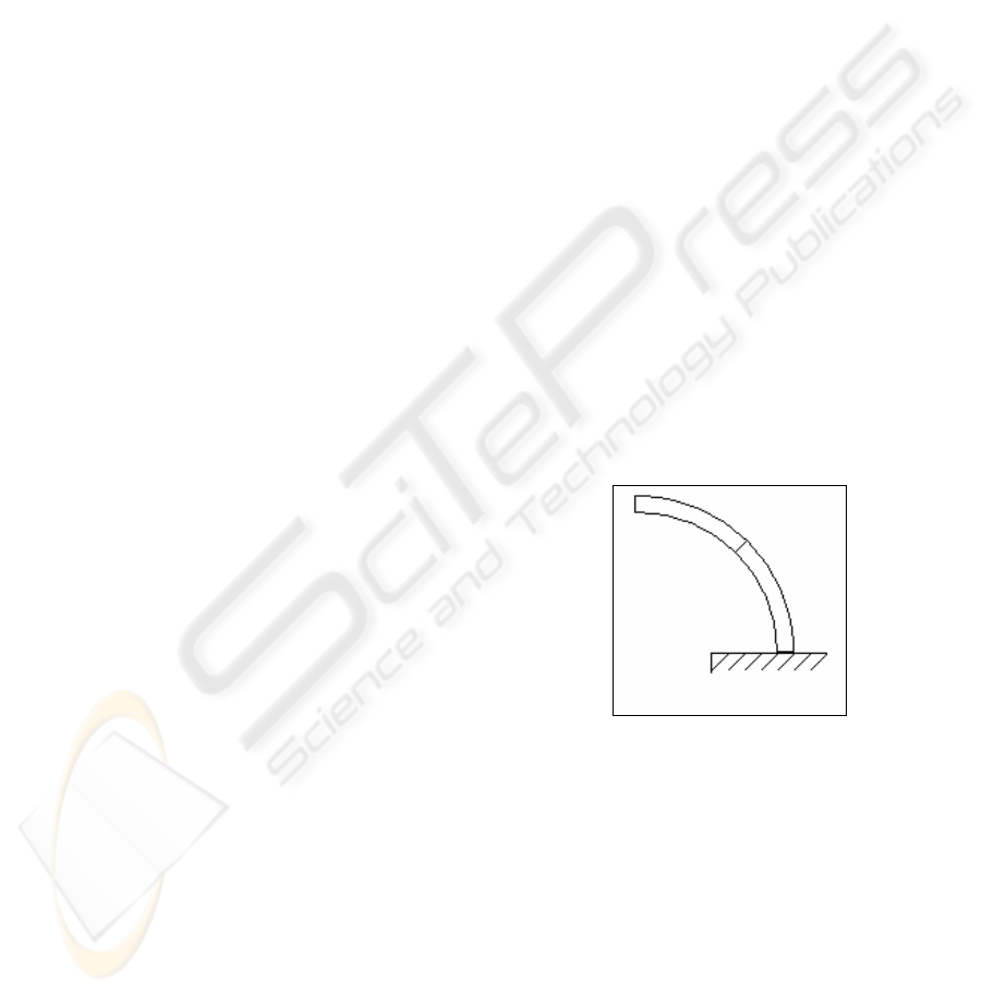
Figure 2 illustrates one possible physical

configuration for the robot where the lengths

and

are equal and the angle formed by each section is

45˚. For this configuration, the first analysis method

is presented, based upon variations in lengths and in

curvatures of up to ±5% of their nominal values.

Figure 3 illustrates the workspace achieved by the

robot if the curvature of the sections is changed by

altering the radius by ±5% while the length of the

sections remains constant.

Figure 2: Physical configuration

In this configuration, only the 2D workspace

plots are presented. Figure 4 illustrates the

workspace when the curvature of the sections is

unchanged while the length of the sections varies

±5% of the nominal length. In Figure 5, both the

curvature and the length have varied up to ±5% of

their nominal values.

EXTENSION VERSUS BENDING FOR CONTINUUM ROBOTS

261

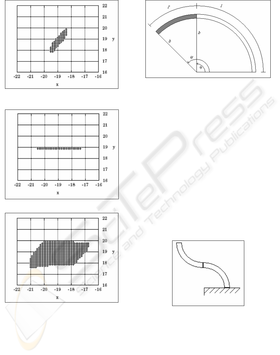
Figure 3: Curvature change only for example of Figure 2

Figure 4: Length change only for example of Figure 2

Figure 5: Length and Curvature change for example of

Figure 2

As can be seen in Figures 3, 4, and 5, changing

the curvature of the sections in concert with the

lengths results in a significantly increased

workspace. Indeed, the workspace achieved by the

combined variations is a form of vector-product of

the length and curvature workspaces.

Figure 6: Changing length for a curved section

As the sections of the robot extend and retract,

the angles formed by the sections (

θ) also change,

even though manipulation was performed on the

length alone. This is an inadvertent effect that comes

from altering the length of a curved section. In

Figure 6, this concept is illustrated for a single

curved section. As the length of the section increases

from

l to l+l`, the radius (which in turn defines the

curvature 1/radius) remains the same while the angle

θ increases to θ ΄.

In Figure 7, we consider a different

configuration. Here, the angle formed by section 2 is

the negative of the angle formed by section 1,

essentially changing the direction of concavity for

section 2. The lengths of the individual sections are

again equal, but the angles formed are (90, -90) for

sections 1 and 2 respectively. The second analysis

method is presented for this configuration, based on

variations around the nominal lengths and curvatures

that change

θ up to ±5 degrees.

Figure 7: Physical configuration

ICINCO 2005 - ROBOTICS AND AUTOMATION

262

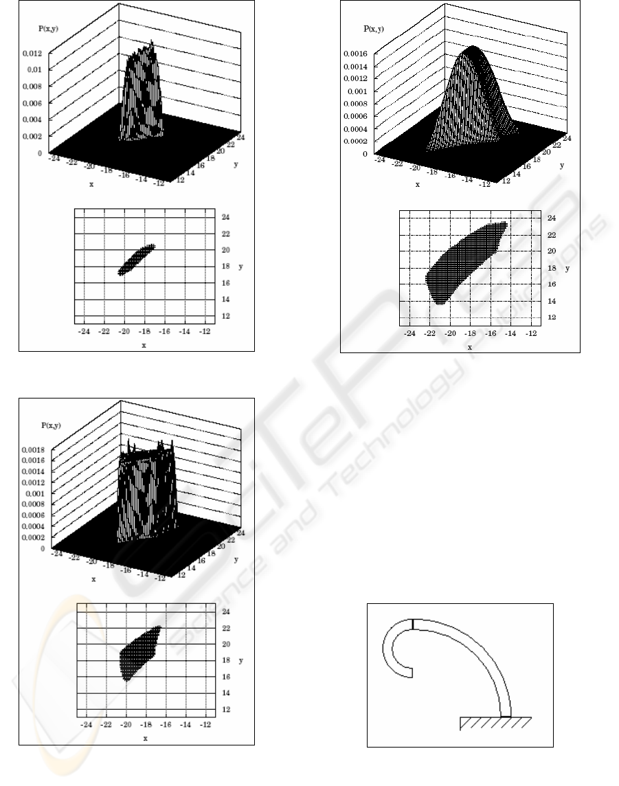
Figure 8: Curvature change only for example of Figure 7

Figure 9: Length change only for example of Figure 7

Figure 10: Length and Curvature change for example of

Figure 7

In Figure 8, the curvatures of the sections have

been changed ±5 degrees respectively. Figure 9

illustrates a change in link length that will change

up to ±5 degrees, and Figure 10 is the workspace

formed when the link length and the curvatures are

changed in concert. Once again, the resultant

workspace in Figure 10 appears as an intuitive

combination of Figures 8 and 9.

In Figure 11, a third configuration is examined.

Here,

= 2 and the angles formed by the length

and curvatures of the sections are (90˚, 180˚)

respectively.

Figure 11: Physical configuration

EXTENSION VERSUS BENDING FOR CONTINUUM ROBOTS

263

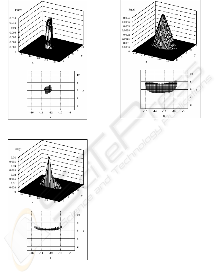
Figure 12: Curvature change only for example of Figure

Figure 13: Length change only for example of Figure 11

Figure 14: Length and Curvature change for example of

Figure 11

Figure 12 illustrates both the workspace and the

PDF generated when the length of the sections vary

such that

θ alters ±5 degrees.

When part of the workspace has a low PDF, as

can be observed in Figures 13 and 14, it indicates

that only a few combinations of the input variables

would allow reaching that part of the workspace.

This relationship could be important with trajectory

planning, among other topics.

In the configurations examined, the workspace

formed from the combined change in the curvatures

and the lengths was significantly larger than the

workspace achieved when only one attribute was

altered. The fact that the resultant workspace

appears as a combination of the two individual

workspaces is also intuitive.

The above examples are typical of the results of

the study, in terms of showing how both bending

and extension significantly affect the workspace, and

in complementary ways. The results also provide the

workspace for a large number of more nonintuitive

configurations. So the approach can also be seen as a

useful tool for task and motion planning.

6 CONCLUSIONS

This paper clearly shows how extension is

complementary to bending in continuum structures,

in terms of workspace enhancement. This is a useful

ICINCO 2005 - ROBOTICS AND AUTOMATION

264

feature that has been taken advantage of by a variety

of animals. The results motivate the inclusion of

extension in future continuum robot designs. Our

current work focuses on the use of the results in this

paper for optimal design and operation of continuum

robots by developing “synergies” from combinations

of extension and bending in the Oct-Arm series of

continuum robots.

ACKNOWLEDGEMENTS

This work supported by DARPA Contract N66001-

C-8043, and by the Spanish Ministry of Science and

Technology under Project TIC2003-09061-C03-02.

REFERENCES

Aoki T., Ochiai A., and Hirose S., 2004. Study on Slime

Robot. In IEEE Int.. Conf. on Robotics and

Automation, New Orleans, pp. 2808-2813.

Blessing M. and Walker I.D., 2004. Novel Continuum

Robots with Variable-Length Sections. In 3

IFAC

Symposium on Mechatronic Systems, Sydney,

Australia, pp. 55-60.

Buckingham R. and Graham A., 2003. Reaching the

unreachable - snake arm robots. In Int. Symposium of

Robotics, Chicago.

Cieslak R. and Morecki A., 1999. Elephant Trunk Type

Elastic Manipulator – A Tool for Bulk and Liquid

Type Materials Transportation. Robotica, vol. 17, pp.

11-16.

Gravagne I.A. and Walker I.D., 2000. On the Kinematics

of Remotely-Actuated Continuum Robots. In IEEE

Int. Conference on Robotics and Automation, San

Francisco, pp. 2544-2550.

Hannan M.W. and Walker I.D., 2003. Kinematics and the

Implementation of an Elephant’s Trunk Manipulator

and Other Continuum Robots. Journal of. Robotic

Systems, 20(2), pp. 45-63.

Hirose S., 1993. Biologically Inspired Robots., Oxford U.

Press.

Immega G. and Antonelli K., 1995. The KSI Tentacle

Manipulator. In IEEE Int. Conference on Robotics and

Automation, pp. 3149-3154.

Jones B. and Walker I.D., 2004. A New Approach to

Jacobian Formulation for Multi-Section Continuum

Robots. In IEEE Int. Conf. on Robotics and

Automation, Barcelona, pp. 3279-3284.

Jones B., McMahan W. and Walker I.D., 2004. Design

and Analysis of a Novel Pneumatic Manipulator. In 3

IFAC Symposium on Mechatronic Systems, Sydney,

Australia, pp. 745-750.

Kier W.M. and Smith K.K., 1985. Tongues, Tentacles,

and Trunks: the Biomechanics of Movement in

Muscular-Hydrostats. Zoological Journal of the

Linnean Society, vol. 83, pp. 307-324.

McMahan W., Jones B., Walker I.D., Chitrakaran V.,

Seshadri A., and Dawson D., 2004. Robotic

Manipulators Inspired by Cephalopod Limbs. In

CDEN Design Conf., Montreal, pp. 1-10.

Moore R.E., 1979, Methods and Applications of Interval

Analysis, SIAM, Philadelphia.

Ohno H. and Hirose S., 2001. Design of Slim Slime Robot

and its Gait of Locomotion. In IEEE/RSJ Int.

Conference on Intelligent Systems, Maui, Hawaii,

USA. pp. 707-715.

Pritts M.B. and Rahn C.D., 2004. Design of an Artificial

Muscle Continuum Robot. In IEEE Int. Conference on

Robotics and Automation, New Orleans, pp. 4742-

4746.

Robinson G. and Davies J.B.C., 1999. Continuum Robots

– A State of the Art. In IEEE Int. Conf. on Robotics

and Automation, pp. 2849– 2854.

Simaan N., Taylor R., and Flint P., 2004. A Dexterous

System for Laryngeal Surgery. In IEEE Int.

Conference on Robotics and Automation, New

Orleans, pp. 351-357.

Suzumori K., Iikura S., Tanakan H., 1991. Development

of Flexible Microactuator and its application to

Robotic Mechanisms. In IEEE Int. Conf. on Robotics

and Automation, pp. 1622-1627.

Takanobu H., Tandai T., and Miura H., 2004. Multi-DOF

Flexible Robot Based on Tongue. In IEEE Int.

Conference on Robotics and Automation, New

Orleans, pp. 2673-2678.

Tsukagoshi H., Kitagawa A., and Segawa M., 2001.

Active Hose: an Artificial Elephant's Nose with

Maneuverability for Rescue Operation. In IEEE Int.

.Conference on Robotics and Automation, Seoul,

Korea, pp. 2454-2459.

Walker I.D. and Carreras C., 2003. Variation of the

Bending Locations within a Robot Manipulator. In

IEEE Int. Conference on Advanced Robotics,

Coimbra, Portugal, pp. 556-561.

Wilson J.F., Li D., Chen Z., and George Jr. R.T., 1993.

Flexible Robot Manipulators and Grippers: Relatives

of Elephant Trunks and Squid Tentacles. Robots and

Biological Systems: Toward a New Bionics?, pp.474-

479.

EXTENSION VERSUS BENDING FOR CONTINUUM ROBOTS

265