IMAGE-BASED AND INTRINSIC-FREE VISUAL NAVIGATION

OF A MOBILE ROBOT DEFINED AS A GLOBAL VISUAL

SERVOING TASK

C. P

erez, N. Garc

ıa-Aracil, J.M. Azor

ın, J.M. Sabater, L. Navarro

R. Saltar

Departamento de Autom

atica, Electr

onica e Inform

atica Industrial Universidad Polit

ecnica de Madrid.

Dept. Ingenier

ıa de Sistemas Industriales. Universidad Miguel Hern

andez.

Avd. de la Universidad s/n. Edif. Torreblanca. 03202 Elche, Spain

Keywords:

Visual servoing, mobile robot navigation, continuous path control.

Abstract:

The new contribution of this paper is the deﬁnition of the visual navigation as a global visual control task which

implies continuity problems produced by the changes of visibility of image features during the navigation. A

new smooth task function is proposed and a continuous control law is obtained by imposing the exponential

decrease of this task function to zero. Finally, the visual servoing techniques used to carry out the navigation

are the image-based and the intrinsic-free approaches. Both are independent of calibration errors which is

very useful since it is so difﬁcult to get a good calibration in this kind of systems. Also, the second technique

allows us to control the camera in spite of the variation of its intrinsic parameters. So, it is possible to modify

the zoom of the camera, for instance to get more details, and drive the camera to its reference position at the

same time. An exhaustive number of experiments using virtual reality worlds to simulate a typical indoor

environment have been carried out.

1 INTRODUCTION

Image-based visual servoing approach is now a well

known control framework (Hutchinson et al., 1996).

A new visual servoing approach, which allows to con-

trol a camera with changes in its intrinsic parame-

ters, has been published in the last years (Malis and

Cipolla, 2000; Malis, 2002c). In both approaches,

the reference image corresponding to a desired po-

sition of the robot is generally acquired ﬁrst (during

an off-line step), and some image features extracted.

Features extracted from the initial image or invariant

features calculated from them are used with those ob-

tained from the desired one to drive back the robot to

its reference position.

The framework for robot navigation proposed is

based on pre-recorded image features obtained during

a training walk. Then, we want that the mobile robot

repeat the same walk by means of image-based and

intrinsic-free visual servoing techniques. The main

contribution of this paper are the deﬁnition of the vi-

sual navigation as a global visual control task. It im-

plies continuity problems produced by the changes of

visibility of image features during the navigation and

the computing of a continuous control law associated

to it.

According to our knowledge, the approximation

proposed to the navigation is totally different and new

in the way of dealing with the features which go in/out

of the image plane during the path and similar to some

references (Matsumoto et al., 1996) in the way of

specifying the path to be followed by the robot.

2 AUTONOMOUS NAVIGATION

USING VISUAL SERVOING

TECHNIQUES

The strategy of the navigation method used in this pa-

per is shown in Figure 1. The key idea of this method

is to divide the autonomous navigation in two stages:

the ﬁrst one is the training step and the second one is

the autonomous navigation step. During the training

step, the robot is human commanded via radio link

or whatever interface and every sample time the robot

acquires an image, computes the features and stores

them in memory. Then, from near its initial position,

the robot repeat the same walk using the reference

features acquired during the training step.

189

Pérez C., García-Aracil N., M. Azorín J., M. Sabater J., Navarro L. and Saltarén R. (2005).

IMAGE-BASED AND INTRINSIC-FREE VISUAL NAVIGATION OF A MOBILE ROBOT DEFINED AS A GLOBAL VISUAL SERVOING TASK.

In Proceedings of the Second International Conference on Informatics in Control, Automation and Robotics - Robotics and Automation, pages 189-195

DOI: 10.5220/0001155301890195

 SciTePress

Mobilerobot:Referencepose

Mobilerobot:Currentpose

Teachingstep

Recording

featuressequence

AutonomousNavigation

basedonrecorded

featuressequence

1.- Acquireimage

2.-Computefeatures

3.-Recordfeatures

Ineachsampletime:

Figure 1: The strategy of the navigation method imple-

mented. First a training step and the autonomous naviga-

tion.

2.1 Control law

As it was mentioned in Section 1, image-based and

intrinsic-free visual servoing approaches (Hutchinson

et al., 1996; Malis and Cipolla, 2000) was used to de-

velop the autonomous navigation of the robot. Both

approaches are based on the selection of a set s of vi-

sual features or a set q of invariant features that has

to reach a desired value s

∗

or q

∗

. Usually, s is com-

posed of the image coordinates of several points be-

longing to the considered target and q is computed as

the projection of s in the invariant space calculated

previously. In the case of our navigation method, s

∗

or q

∗

is variable with time since in each sample time

the reference features is updated with the desired tra-

jectory of s or q stored in the robot memory in order

to indicate the path to be followed by the robot.

To simplify in this section, the formulation pre-

sented is only referred to image-based visual ser-

voing. All the formulation of this section can be

applied directly to the invariant visual servoing ap-

proach changing s by q. The visual task function

(Samson et al., 1991) is deﬁned as the regulation of

an global error function instead of a set of discrete

error functions (Figure 2):

e = C(s − s

∗

(t)) (1)

The derivative of the task function,considering C

constant, will be:

˙e = C(˙s − ˙s

∗

) (2)

It is well known that the interaction matrix L , also

called image jacobian, plays a crucial role in the de-

sign of the possible control laws. L is deﬁned as:

s = L v (3)

where v = (V

, ω

) is the camera velocity screw

(V and ω represent its translational and rotational

component respectively).

Plugging the equation (3) in (2) we obtain:

˙e = CLv − C ˙s

∗

(4)

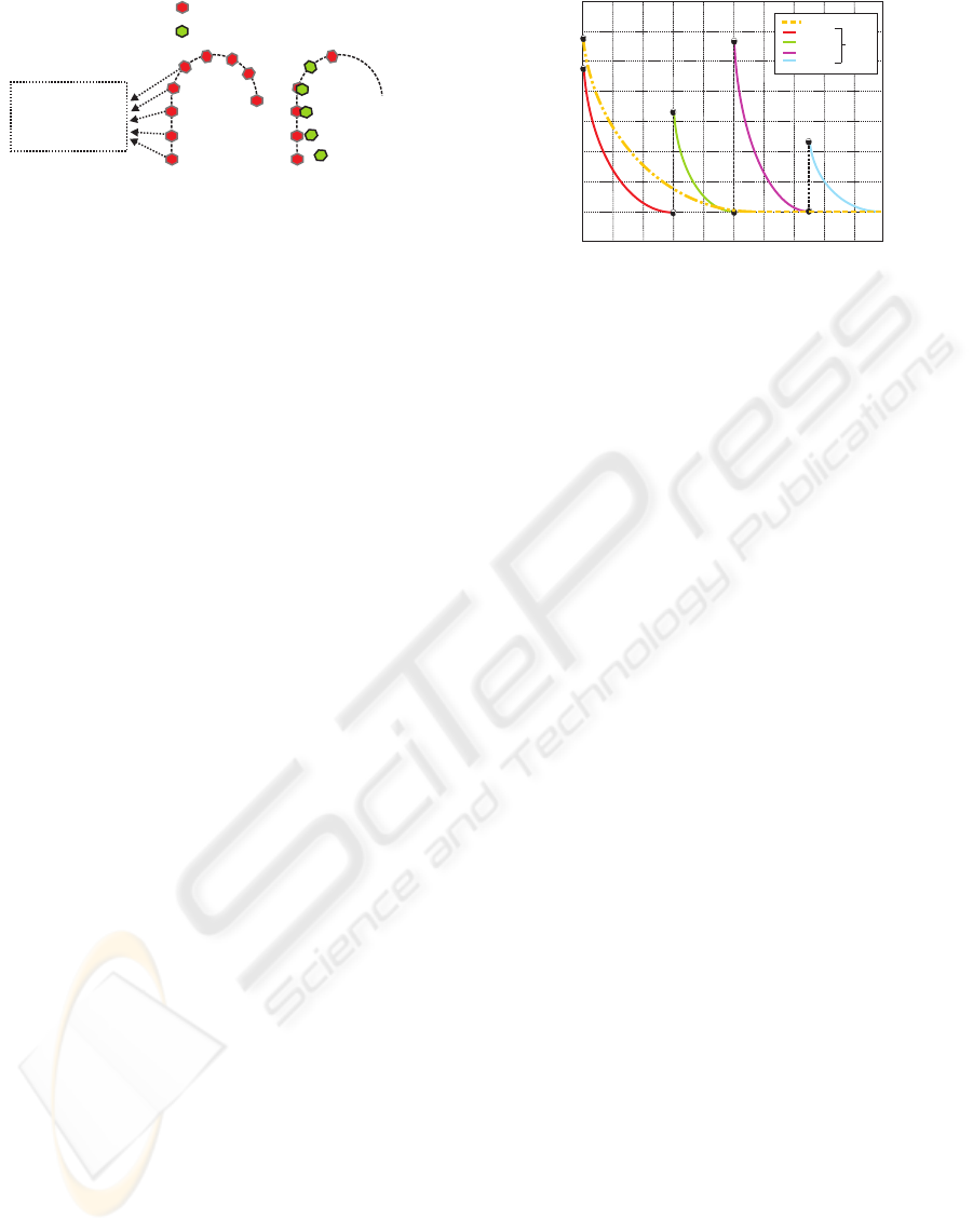
Error

Iterations

Global Task

Sub-Task1

Sub-Task2

Sub-Task3

Sub-Task4

Discreet

Total

Task

Figure 2: Navigation as a global task vs discretization of the

navigation task

A simple control law can be obtained by imposing

the exponential convergence of the task function to

zero:

˙e = −λ e so CLv = −λ e + C ˙s

∗

(5)

where λ is a positive scalar factor which tunes the

speed of convergence:

v = −λ (CL)

−1

e + (CL)

−1

C ˙s

∗

(6)

if C is setting to L

, then (CL) > 0 and the task

function converge to zero and, in the absence of local

minima and singularities, so does the error s − s

∗

. Fi-

nally substituting C by L

in equation (6), we obtain

the expression of the camera velocity that is sent to

the robot controller:

v = −λ L

(s − s

∗

(t)) + L

˙s

∗

(7)

Remember that the whole formulation is directly

applicable to the invariant visual servoing approach

changing s by q. As will be shown in the next section,

discontinuities in the control law will be produced by

the appearance/disappearance of image features dur-

ing the navigation of the robot. The answer to the

question: why are these discontinuities produced and

their solution are presented in the following section.

3 DISCONTINUITIES IN VISUAL

NAVIGATION

In this section, we describe more in details the dis-

continuity problem that occurs when some features go

in/out of the image during the vision-based control. A

simple simulation illustrate the effects of the disconti-

nuities on the control law and on the performances of

the visual servoing. The navigation of a mobile robot

is a typical example where this kind of problems are

produced.

ICINCO 2005 - ROBOTICS AND AUTOMATION

190

(a) Croquis of the autonomous navigation of the robot

1 2

Imageplaneattimek

Imageplaneattimek+1

attimek+1

Referencefeatures

Currentfeatures

s=( ,s, ,s,s,s,s)s s

1 32 4 5 6 7

s=( , )

* T

s, ,s,s,s,s

* * * * *

2 4 5 6 7

Remove

s=(s,s,s,s,s )

2 4 5 6 7

, s,s,s,s

8 9 10 11

Add

s=(s,s,s,s,s, )

* * * * * * T

2 4 5 6 7

s,s,s,s

* * * *

8 9 10 11

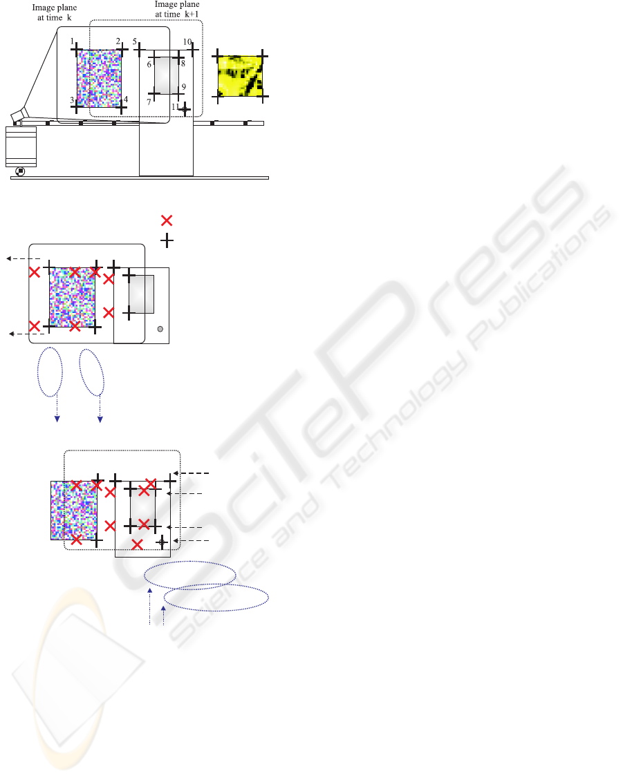
(b) Appearance/Disappearance of image features

from time k to k+1

Figure 3: Navigation of a mobile robot controlled by visual

servoing techniques.

3.1 What happens when features

appear or disappear from the

image plane?

During autonomous navigation of the robot, some

features appear or disappear from the image plane so

they will must be added to or removed from the visual

error vector (Figure 3). This change in the error vec-

tor produces a jump discontinuity in the control law.

The magnitude of the discontinuity in control law de-

pends on the number of the features that go in or go

out of the image plane at the same time, the distance

between the current and reference features, and the

pseudoinverse of interaction matrix.

In the case of using the invariant visual servoing ap-

proach to control the robot, the effect produced by the

appearance/disappearance of features could be more

important since the invariant space Q used to compute

the current and the reference invariant points(q, q

∗

)

changes with features(Malis, 2002c).

4 CONTINUOUS CONTROL LAW

FOR NAVIGATION

In the previous section, the continuity problem of the

control law due to the appearance/disappearance of

features has been shown. In this section a solution is

presented. The section is organized as follows. First,

the concept of weighted features is deﬁned. Then, the

deﬁnition of a smooth task function is presented. Fi-

nally, the reason to reformulate the invariant visual

servoing approach and its development is explained.

4.1 Weighted features

The key idea in this formulation is that every feature

(points, lines, moments, etc) has its own weight which

may be a function of image coordinates(u,v) and/or a

function of the distance between feature points and

an object which would be able to occlude them, etc

(Garc

ıa et al., 2004). To compute the weights, three

possible situations must be taking into account:

4.1.1 Situation 1: Changes of visibility through

the border of the image (Zone 2 in Figure 4

To anticipate the changes of visibility of features

through the border, a total weight Φ

is computed

as the product of the weights of the current and ref-

erence features which are function of their position in

the image (γ

, γ

∗

). The weight γ

= γ

· γ

computed using the deﬁnition of the function γ

(x)

(γ

= γ

) and γ

= γ

) respectively) (Garc

ıa

et al., 2004).

4.1.2 Situation 2: The sudden appearance of

features on the center of the image (Zone 1

in Figure 4 b)

To take into account this possible situation, every new

features (current and reference) must be checked pre-

IMAGE-BASED AND INTRINSIC-FREE VISUAL NAVIGATION OF A MOBILE ROBOT DEFINED AS A GLOBAL

VISUAL SERVOING TASK

191

Zona1

Zona2

Zone1

Zone2

Zone1

Zone2

Image

Zone1

Zone2

Zone1

Zone2

(a) Border of the image

MobileRobot(Teachingstep)

MobileRobot(InitialPose)

Zone2

Image

(b) Center of the image

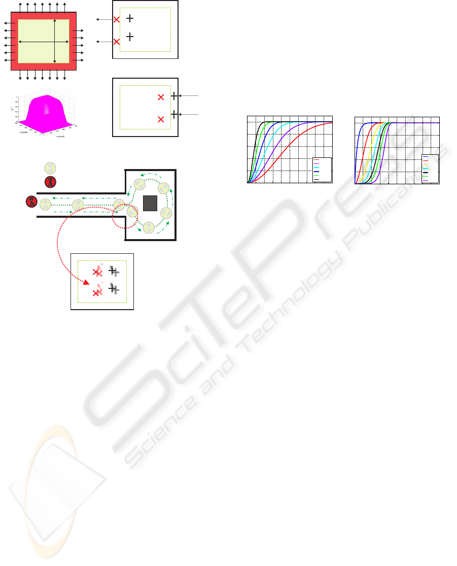
Figure 4: Appearance/Disappearance of image features

through the border and the center of the image during the

navigation of the mobile robot.

viously to known if they are in Zone 2 or Zone 1. If

the new features are in Zone 2, the appearance of the

features are considered in Situation 1. If they are in

Zone 1, a new weight function must be deﬁned to add

these new features in a continuos way.

The weight function proposed Φ

is a exponential

function that tends to 1, reaching its maximum after

a certain number of steps which can be modiﬁed with

the α and β parameters (Figure 5):

(t) = 1 − e

−α · t

α, β > 0 (8)

4.1.3 Situation 3: The sudden disappearance of

features on the center of the image because

of a temporal or deﬁnitive occlusion (Zone

1 in Figure 4 b)

In this situation, the occlusions produced in the teach-

ing step on the Zone 1 are only considered since they

can be easily anticipated by the observation of refer-

ence features vector prerecorded previously.

To take into account this possible situation, a new

weight function must be deﬁned to remove these fea-

tures from the current and reference vector in a con-

tinuos way. The weight function proposed Φ

is a

exponential function that tends to 0, reaching its min-

imum after a certain number of steps which can be

modiﬁed with the ν and σ parameters:

(t) = e

−ν · t

ν, σ > 0 (9)

0 20 40 60 80 100 120 140 160 180 200

0.2

0.4

0.6

0.8

1.1

−2

α = 1

α = 2

α = 4

α = 8

α = 16

α = 32

β = 2

(a) Φ

(α)

0 20 40 60 80 100 120 140 160 180 200

0.2

0.4

0.6

0.8

−2

β = 1

β = 2

β = 3

β = 4

β = 5

β = 6

β = 8

α = 16

(b) Φ

(β)

Figure 5: Plotting Φ

in function of α and β.

4.1.4 Global weight function Φ

In this section, a global weight function Φ

which in-

cludes the three possible situations commented before

is presented. This function is deﬁned as the product

of the three weight functions (Φ

, Φ

y Φ

) which

takes into account the three possible situations:

= Φ

· Φ

where Φ

∈ [0, 1] (10)

4.2 Smooth Task function

Suppose that n matched points are available in the

current image and in the reference features stored.

Everyone of these points(current and reference) will

have a weight Φ

which can be computed as it’s shown

in the previous subsection 4.1. With them and their

weights, a task function can be built (Samson et al.,

1991):

e = CW (s − s

∗

(t)) (11)

where W is a (2n × 2n) diagonal matrix where its

elements are the weights Φ

of the current and refer-

ence features multiplied by the weights of the refer-

ence features.

The derivate of the task function will be:

˙e = CW (˙s − ˙s

∗

) + (C

W +

CW)(s − s

∗

(t)) (12)

Plugging the equation (˙s = L v) in (12) we obtain:

˙e = CW (Lv− ˙s

∗

)+(C

W+

CW)(s−s

∗

(t)) (13)

A simple control law can be obtained by imposing the

exponential convergence of the task function to zero

ICINCO 2005 - ROBOTICS AND AUTOMATION

192

(˙e = −λe), where λ is a positive scalar factor which

tunes the speed of convergence:

v = −λ (CWL)

−1

e + (CWL)

−1

CW˙s

∗

− (CWL)

−1

W +

CW) (s − s

∗

(t))(14)

if C is setting to (W

∗

)

,then (CWL) > 0 and

the task function converge to zero and, in the absence

of local minima and singularities, so does the error

s−s

∗

. In this case, C is constant and therefore

C = 0.

Finally substituting C by (W

∗

)

in equation (14),

we obtain the expression of the camera velocity that

is sent to the robot controller:

v = −(W

∗

)

(λ W +

W) (s − s

∗

(t)) +

+ (W

∗

)

W˙s

∗

(15)

4.3 Visual servoing techniques

The visual servoing techniques used to carry out the

navigation are the image-based and the intrinsic-free

approaches. In the case of image-based visual ser-

voing approach, the control law (15) is directly ap-

plicable to assure a continuous navigation of a mobile

robot. On the other hand, when the intrinsic-free ap-

proach is used, this technique must be reformulated to

take into account the weighted features.

4.3.1 Intrinsic-free approach

The theoretical background about invariant visual ser-

voing can be extensively found in (Malis, 2002b;

Malis, 2002c). In this section, we modify the ap-

proach in order to take into account weighted features

(Garc

ıa et al., 2004).

Basically, the weights Φ

deﬁned in the previous

subsection must be redistributed(γ

) in order to be

able to build the invariant projective space Q

where

the control will be deﬁned.

Similarly to the standard intrinsic-free visual ser-

voing, the control of the camera is achieved by

stacking all the reference points of space Q

in a

(3n×1) vector s

∗

(ξ

∗

) = (q

∗

(t), q

∗

(t), · · · , q

∗

(t)).

Similarly, the points measured in the current cam-

era frame are stacked in the (3n×1) vector s(ξ) =

(t), q

(t), · · · , q

(t)). If s(ξ) = s

∗

(ξ

∗

) then

ξ = ξ

∗

and the camera is back to the reference po-

sition whatever the camera intrinsic parameters.

In order to control the movement of the camera,

we use the control law (15) where W depends on

the weights previously deﬁned and L is the interac-

tion matrix. The interaction matrix depends on cur-

rent normalized points m

(ξ) ∈ M (m

can be com-

puted from image points m

= K

−1

), on the in-

variant points q

(ξ) ∈ Q

, on the current depth dis-

tribution z(ξ) = (Z

, Z

, ..., Z

) and on the current

redistributed weights γ

. The interaction matrix in the

weighted invariant space (L

q i

= T

−C

))is

obtained like in (Malis, 2002a) but the term C

must be recomputed in order to take into account the

redistributed weights γ

5 EXPERIMENTS IN A VIRTUAL

INDOOR ENVIRONMENT

Exhaustive experiments have been carried out using

a virtual reality tool for modeling an indoor envi-

ronment. To make more realistic simulation, errors

in intrinsic and extrinsic parameters of the camera

mounted in the robot and noise in the extraction of

image features have been considered. An estimation

K of the real matrix K has been used with an error

of 25% in focal length and a deviation of 50 pixels

in the position of the optical center. Also an esti-

mation

of the camera pose respect to the ro-

bot frame has been computed with a rotation error of

uθ = [3.75 3.75 3.75]

degr ees and translation er-

ror of t = [2 2 0]

cm. An error in the extraction of

current image features has been considered by adding

a normal distribution noise to the accurate image fea-

tures extracted.

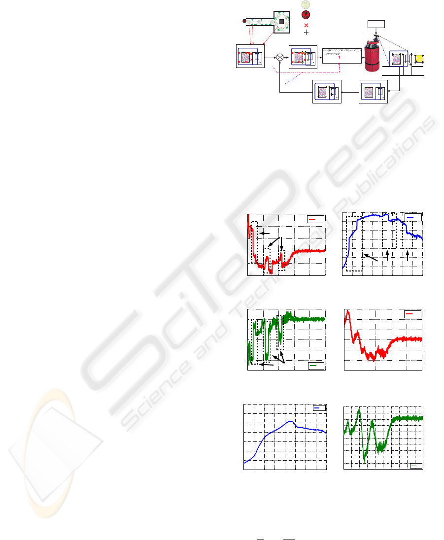
In Figure 7, the control signals sent to the robot

controller using the classical image-based approach

and the image-based approach with weighted features

are shown. In Figure 7 (a,b,c), details of the control

law using the classical image-based approach, where

the discontinuities can be clearly appreciated, are pre-

sented. To show the improvements of the new formu-

lation presented in this paper, the control law using

the image-based with weighted features can be seen

in Figure 7 (d,e,f).

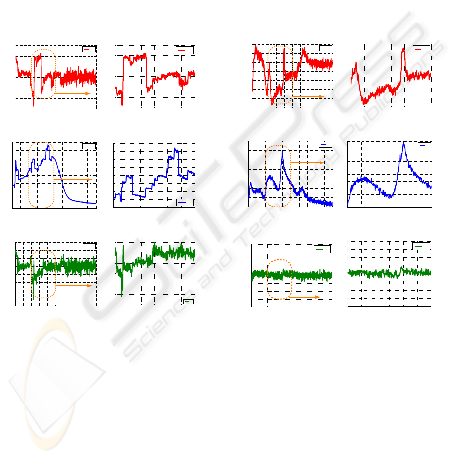
The same experiment, but in this case using the

intrinsic-free visual servoing approach, is performed.

In Figure 8 , the control signals sent to the robot con-

troller using the intrinsic-free approach and some de-

tails, where the discontinuities can be clearly appre-

ciated, are shown. The improvements of the new for-

mulation of the intrinsic-free approach with weighted

features are presented in Figure 9. The same details

of the control law shown in Figure 8 are presented

in Figure 9. Comparing both ﬁgures and their details,

the continuity of the control law is self-evident despite

of the noise in the extraction of image features.

Also in (Garc

ıa et al., 2004), a comparison between

this method and a simple ﬁltration of the control law

was presented. The results presented in that paper cor-

roborate that the new approach with weighted features

to the problem works better than a simple ﬁlter of the

control signals.

IMAGE-BASED AND INTRINSIC-FREE VISUAL NAVIGATION OF A MOBILE ROBOT DEFINED AS A GLOBAL

VISUAL SERVOING TASK

193

6 CONCLUSIONS

In this paper the originally deﬁnition of the visual

navigation as a global visual control task is pre-

sented. It implies continuity problems produced by

the changes of visibility of image features during the

navigation which have been solved by the deﬁnition

of a smooth task function and a continuous control

law obtained from it. The results presented corrobo-

rate that the new approach is continuous, stable and

works better than a simple ﬁlter of the control signals.

The validation of this results with a real robot is on

the way by using a B21r mobile robot from iRobot

company.

REFERENCES

Garc

ıa, N., Malis, E., Reinoso, O., and Aracil, R. (2004).

Visual servoing techniques for continuous navigation

of a mobile robot. In 1st International Conference

on Informatics in Control, Automation and Robotics,

volume 1, pages 343–348, Setubal, Portugal.

Hutchinson, S. A., Hager, G. D., and Corke, P. I. (1996). A

tutorial on visual servo control. IEEE Trans. Robotics

and Automation, 12(5):651–670.

Malis, E. (2002a). Stability analysis of invariant visual

servoing and robustness to parametric uncertainties.

In Second Joint CSS/RAS International Workshop on

Control Problems in Robotics and Automation, Las

Vegas, Nevada.

Malis, E. (2002b). A uniﬁed approach to model-based

and model-free visual servoing. In European Confer-

ence on Computer Vision, volume 2, pages 433–447,

Copenhagen, Denmark.

Malis, E. (2002c). Vision-based control invariant to camera

intrinsic parameters: stability analysis and path track-

ing. In IEEE International Conference on Robotics

and Automation, volume 1, pages 217–222, Washing-

ton, USA.

Malis, E. and Cipolla, R. (2000). Self-calibration of zoom-

ing cameras observing an unknown planar structure.

In Int. Conf. on Pattern Recognition, volume 1, pages

85–88, Barcelona, Spain.

Matsumoto, Y., Inaba, M., and Inoue, H. (1996). Vi-

sual navigation using view-sequenced route represen-

tation. In IEEE International Conference on Robotics

and Automation (ICRA’96), volume 1, pages 83–88,

Minneapolis, USA.

Samson, C., Le Borgne, M., and Espiau, B. (1991). Robot

Control: the Task Function Approach. volume 22 of

Oxford Engineering Science Series.Clarendon Press.,

Oxford, UK, 1st edition.

RobotControl

Zoom

Referencefeatures

recordedinrobotmemory

s*(t)

ReferenceFeatures

CurrentFeatures

Features

1 2

ImagePlane

ImageAdquisition

ImagePlane

1 2

ImagePlane

FeatureError

1 2

MobileRobot(ReferencePose). Teachingstep

MobileRobot(CurrentPose)

.....

Figure 6: Block diagram of the controller proposed

0 200 400 600 800 1000

−0.01

−0.005

0.005

0.01

0.015

Iterations number

Discontinuities

(a) ω

0 50 100 150 200 250 300 350 400

0.52

0.54

0.56

0.58

0.6

0.62

0.64

0.66

Iterations number

Discontinuities

(b) v

0 200 400 600 800 1000

−0.025

−0.02

−0.015

−0.01

−0.005

0.005

Iterations number

Discontinuities

0 200 400 600 800 1000

−0.015

−0.01

−0.005

0.005

0.01

0.015

Iterations number

(d) ω

0 50 100 150 200 250 300 350 400

0.4

0.45

0.5

0.55

0.6

0.65

0.7

0.75

Iterations number

(e) v

0 100 200 300 400 500 600 700 800 900 1000

−0.04

−0.035

−0.03

−0.025

−0.02

−0.015

−0.01

−0.005

0.005

0.01

Iterations number

(f) v

Figure 7: Control law: Classical image-based approach (a-

b-c) and image-based approach with weighted features (d-e-

f).The translation and rotation speeds are measured respec-

tively in

and

deg

ICINCO 2005 - ROBOTICS AND AUTOMATION

194

0 100 200 300 400 500 600 700 800 900 1000

−0.015

−0.01

−0.005

0.005

0.01

0.015

Iterations number

Detail

(a) ω

200 250 300 350 400 450 500

−0.015

−0.01

−0.005

0.005

0.01

0.015

Iterations number

(b) Details

0 100 200 300 400 500 600 700 800 900 1000

0.1

0.2

0.3

0.4

0.5

0.6

0.7

0.8

Iterations number

Detail

200 250 300 350 400 450 500

0.4

0.45

0.5

0.55

0.6

0.65

0.7

0.75

0.8

Iterations number

(d) Details

0 100 200 300 400 500 600 700 800 900 1000

−0.025

−0.02

−0.015

−0.01

−0.005

0.005

0.01

0.015

Iterations number

Detail

(e) v

200 250 300 350 400 450 500

−0.025

−0.02

−0.015

−0.01

−0.005

0.005

Iterations number

(f) Details

Figure 8: Discontinuities in the control law: Intrinsic-free

approach.

0 100 200 300 400 500 600 700 800 900 1000

−0.025

−0.02

−0.015

−0.01

−0.005

0.005

0.01

Iterations number

Detail

(a) ω

200 250 300 350 400 450 500

−0.025

−0.02

−0.015

−0.01

−0.005

0.005

0.01

Iterations number

(b) Details

0 100 200 300 400 500 600 700 800 900 1000

0.2

0.4

0.6

0.8

1.2

1.4

Iterations number

Detail

200 250 300 350 400 450 500

0.2

0.3

0.4

0.5

0.6

0.7

0.8

0.9

1.1

1.2

Iterations number

(d) Details

0 200 400 600 800 1000

−0.4

−0.3

−0.2

−0.1

0.1

0.2

0.3

0.4

Iterations number

Detail

(e) v

200 250 300 350 400 450 500

−0.4

−0.3

−0.2

−0.1

0.1

0.2

0.3

0.4

Iterations number

(f) Details

Figure 9: Continuous control law: Intrinsic-free approach

with weighted features.

IMAGE-BASED AND INTRINSIC-FREE VISUAL NAVIGATION OF A MOBILE ROBOT DEFINED AS A GLOBAL

VISUAL SERVOING TASK

195