A GRAPHICAL REVIEW OF NOISE-INSTABILITY
CHARA
CTERIZATION IN ELECTRONIC SYSTEMS
Juan Jos
´
e Gonz
´
alez de la Rosa
Univ. C
´
adiz. Electronics Area, EPSA. Ram
´
on Puyol S/N. E-11202-Algeciras-Spain
Isidro Lloret Galiana
Univ. C
´
adiz. Dpt. Computer Science, EPSA. Ram
´
on Puyol S/N. E-11202-Algeciras-Spain
Carlos Garc
´
ıa Puntonet
Univ. Granada. Dept. ATC, ESII. Periodista Daniel Saucedo. E-18071-Granada-Spain
V
´
ıctor Pallar
´
es L
´
opez
Univ. C
´
ordoba. Dept. Electronics, Campus Rabanales. A. Einstein. C-2. E-14071. C
´
ordoba. Spain
Keywords:
Allan deviation, enveloping curves, frequency stability, GPS-receiver, noise processes, traceable calibration.
Abstract:
A thorough study of the noise processes characterization is made with simulated data by means of our non-
classical estimators. Individual and hybrid noise sequences, previously generated by seed functions, have
been used to obtain a set of characterization graphs identifying the noise type by mean of the enveloping
curve. It is also shown the case of a hidden noise. An real test situation is presented which involves a traceable
characterization via a GPS receiver.
1 INTRODUCTION
Noise affects short-term stability of clocks and oscil-
lators of systems in a broad range of technical fields
like communications, instrumentation and medicine.
The relationship between the causes and the differ-
ent noise processes is continuously being reviewed
(Vig, 2001). Random oscillator instabilities are linked
to the environment (temperature changes, vibrations,
shock and electromagnetic fields) and to the guts of
the electronics components (thermal noise, internal ir-
regularities in the xtal and the semiconductor devices,
and surface imperfections).
Numerous works have provided the users with use-
ful analytical tools with the aim of getting the com-
pleteness of the calibration procedure (Allan, 1987),
(Rutman and Walls, 1991). Multivariance analysis al-
lows getting higher measurement accuracy (Vernotte,
1993) in estimating the uncertainties in order to better
distinguish the different types of noises.
In this work we have summarized the subject to
have an unified practical frame, understandable in
multidisciplinary engineering projects. An analysis
of the noise processes is performed to provide an
easy-going review of short term instability character-
ization, by analyzing the slopes of the AVAR
1
and
1
Allan variance or two-sample Allan variance
MVAR
2
in the log-log curves. Noise time series have
been simulated and estimators of the variances have
been programmed with the aim of having a thorough
vision of the time-domain slopes when compared to
former works: (Howe et al., 1999), (Allan, 1987),
(Rutman and Walls, 1991), (Vernotte, 1993), (Vig,
2001).
The paper is structured as follows: in Section 2
we review the oscillators independent noise processes
and the methods used to identify them; Section 3
shows the simulation results concerning time-domain
stability characterization. The concept of enveloping
curve is introduced herein withe the objective of char-
acterizing the effects of different simultaneous noise
processes. A real case of short-term characteriza-
tion procedure and its associated conclusions are pre-
sented in Section 4. In this section, we consider a
precision function generator as device under test in a
GPS-traceable characterization.
2 CLASSICAL NOISE MODELS
It is a customary situation to deal with unperfect sig-
nals which contain additive noise. The instantaneous
2
Modified Allan variance
310
José González de la Rosa J., Lloret Galiana I., García Puntonet C. and Pallarés López V. (2005).
A GRAPHICAL REVIEW OF NOISE-INSTABILITY CHARACTERIZATION IN ELECTRONIC SYSTEMS.
In Proceedings of the Second International Conference on Informatics in Control, Automation and Robotics - Signal Processing, Systems Modeling and
Control, pages 310-315
DOI: 10.5220/0001154903100315
Copyright
c
 SciTePress

output voltage of an oscillator can be expressed as:
v(t) = [V
o
+ ε(t)] sin [2πν
0
t + φ(t)] , (1)
where V
o
is the nominal peak voltage amplitude, ε(t)
is the deviation from the nominal amplitude, ν
0
is the
name-plate frequency, and φ(t) is the phase deviation
from the ideal phase 2πν
0
t. Changes in the peak value
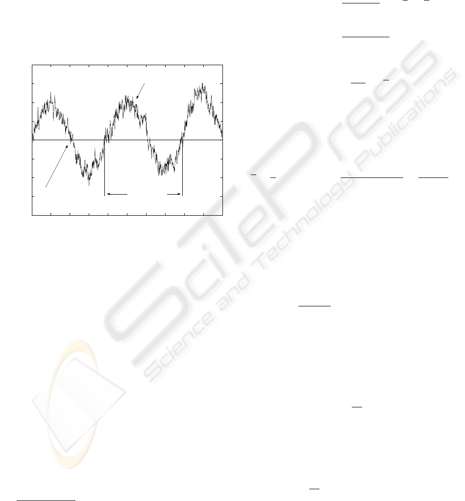
of the signal is the amplitude instability. Fluctuations
in the zero crossings of the voltage is the phase insta-
bility. The so-called frequency instability is depicted
by the fluctuations in the period of the voltage. The
situation is depicted in figure 1
3
.
0 0.01 0.02 0.03 0.04 0.05 0.06 0.07 0.08 0.09 0.1
-2
-1.5
-1
-0.5
0
0.5
1
1.5
2
Time (s)
Voltage (V)
Amplitude instability
Phase instability
Frequency instability
Figure 1: Simulated types of instabilities in a 25 Hz si-
nusoidal output with additive noise. The noise process has
a power spectral density proportional to the inverse of the
frequency (flicker phase modulation).
The impacts of oscillator noise and the causes of
short term instabilities have been described in many
research works and tutorials like (Howe et al., 1999),
(Vig, 2001) and (Sullivan et al., 1990). The short-term
stability measures most frequently found on oscillator
specification sheets is the two-sample deviation, also
called Allan deviation, σ
2
y
(τ).
Classical variance in non-stationary noise
processes don’t converge to concrete values. It
diverges for some noise processes, such as random
walk, i.e., the variance increases with increasing
number of data points. This is the reason whereby
non-classical statistics are used to characterize short
term instability.
AVAR and MVAR have proven their adequacy
in characterizing frequency phase and instabilities.
These easy-to-compute variances converge for all
noise processes observed in precision frequency
sources, have a straightforward relationship to power
3
A similar example was provided by Prof. Eva Ferre-
Pikal (Univ. of Wyoming) and used by John R. Vig in (Vig,
2001).
law spectral density of noise processes, and are faster
and more accurate in than the FFT (Lesage and Ayi,
1984).
The estimates of AVAR and MVAR for a given cali-
bration time τ for a m-data series of phase differences,
x, are given by equations 2 and 3, (Greenhall, 1988):
AV AR ≡ σ
2
y
(τ, m) =
1
2(m − 1)
m
X
j=2

y
j
− y
j−1

2
=
1
2τ
2
(m − 1)
m
X
j=2

∆
2
τ
x(jτ )

2
(2)
MV AR ≡
1
2τ
2
h∆
2
τ
xi
2
, (3)
where the bar over x denotes the average in the
time interval τ (averaging time), and ∆
2
τ
x = x
i+2
−
2x
i+1
+ x
i
, is the so called second difference of
x. The fractional frequency deviation is the relative
phase difference in an interval τ. It is defined by equa-
tion 4:
y =
1
τ
Z
t
t−τ
y(s)ds =
x(t) − x(t − τ )
τ
=
∆
τ
x(t)
τ
.
(4)
Non-classical statistics estimators, defined above, in
equations 2 and 3, for non-stationary series charac-
terization, give an average dispersion of the fractional
frequency deviation due to the noise processes cou-
pled to the oscillator. As a consequence time do-
main instability (two-sample variance) is related to
the noise spectral density via (Rutman and Walls,
1991):
σ
2
y
(τ) =
2
(πν
0
τ)
2
Z
f
h
0
S
φ
(f)sin
4
(πfτ)df, (5)
where ν
0
is the carrier frequency and f is the Fourier
frequency (the variable), and f
h
is the band-width of
the measurement system. S
φ
(f) is the spectral den-
sity of phase deviations, which is in turn related to
the spectral density of fractional frequency deviations
by(Rutman and Walls, 1991):
S
φ
(f) =
ν
2
0
f
2
S
y
(f), (6)
The classical power-law noise model is a sum of the
five common spectral densities. The model can be de-
scribed by the one-sided phase spectral density S
φ
(f)
via (IEEE, 1988), (Greenhall, 1988):
S
φ
(f) =
ν
2
0
f
2
2
X
α=−2
h
α
f
α
= ν
2
0
4
X
β=0
h
β
f
β
, (7)
for 0 ≤ f ≤ f
h
. Where, again, f
h
is the high-
frequency cut-off of the measurement system (the
A GRAPHICAL REVIEW OF NOISE-INSTABILITY CHARACTERIZATION IN ELECTRONIC SYSTEMS
311

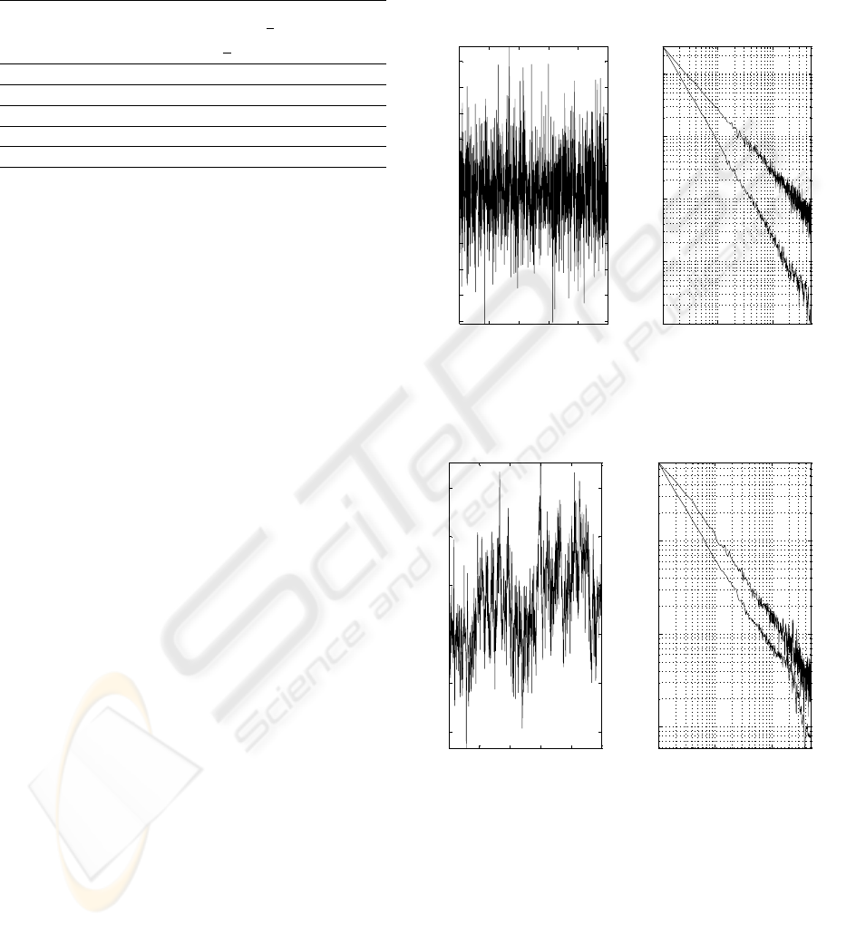
Table 1: Noise processes characterized by the time and fre-
quency domain slopes. Up to bottom: random walk fre-
quency modulation, flicker frequency modulation, white
frequency modulation, flicker phase modulation, white
phase modulation.
AVAR MVAR
S
y
(f) S
φ
(f) σ
y
(τ) ∼ |τ|
µ
2
σ
y
(τ) ∼ |τ|
µ
′
α β = α − 2
µ
2
µ
′
−2 −4 0.5 1 (0.5)
−1 −3 0 0 (0)
0 −2 −0.5 −1 (−0.5)
1 −1 −1 −2 (−1)
2 0 −1 −3 (−1.5)
band-width); h
α
and h
β
are constants which rep-
resent, respectively, the independent characteristic
models of oscillator frequency and phase noise (Al-
lan, 1987), (IEEE, 1988), (Greenhall, 1988).
For integer values (the most common case) we have
the following approximate expression:
σ
y
(τ) ∼ τ
µ/2
, (8)
where µ = −α − 1, for −3 ≤ α ≤ 1; and µ ≈ −2
for α ≥ 1. In the case of the modified Allan variance,
the time-domain instability can be approximated via:
Modσ
y
(τ) ∼ τ
µ
′
(9)
Hereinafter we use expressions 8 and 9 for analyzing
noise in these work.
3 TIME DOMAIN STABILITY
CHARACTERIZATION CURVES
Equations 8 and 9 are used to make the graphical
representation of σ
y
(τ) vs. τ, and lets us infer the
noise processes which causes frequency instability by
means of measuring the slope in a log-log graph (Rut-
man and Walls, 1991), (Wei, 1997). These functional
characteristics of the independent noise processes are
widely used in modelling frequency instability of os-
cillators. Table 1 shows the experimental criteria
adopted in the main references. In the second column
or MVAR we have picked up two different criteria ac-
cording to the references (Rutman and Walls, 1991)
and (Lesage and Ayi, 1984), respectively. We have
kept the notation in the works (Rutman and Walls,
1991) and (Lesage and Ayi, 1984) for µ/2 and µ
′
,
respectively.
The five noise processes have been modelled and
VAR and MVAR have been calculated. Hereinafter
we show the simulation results of the time-series and
their associated VAR and MVAR graphs. From this
simulations we adopt the criteria depicted in the sec-
ond column of MVAR in table 1. Figures 2-6 show
the simulations results. Each data sequence contains
4096 points for a time resolution of τ = 10
−4
s. Al-
lan deviation curves have been depicted for averaging
times τ = n × τ
0
, with n ∈ [1, 500].
0.02 0.04 0.06 0.08 0.1
-0.05
-0.04
-0.03
-0.02
-0.01
0
0.01
0.02
0.03
0.04
0.05
Time (s)
Amplitude (V)
White phase modulation
10
-4
10
-3
10
-2
10
-2
10
-1
10
0
10
1
10
2
log(tau)
log(sigma)
AVAR and MVAR; beta=0
Figure 2: Characterization of a noise process corresponding
to β = 0.
0.02 0.04 0.06 0.08 0.1
-2
-1
0
1
2
3
x 10
-3
Time (s)
Amplitude (V)
Flicker phase mod.
10
-4
10
-3
10
-2
10
-2
10
-1
10
0
log(tau)
log(sigma)
AVAR and MVAR; beta=-1
Figure 3: Characterization of a noise process corresponding
to β = −1.
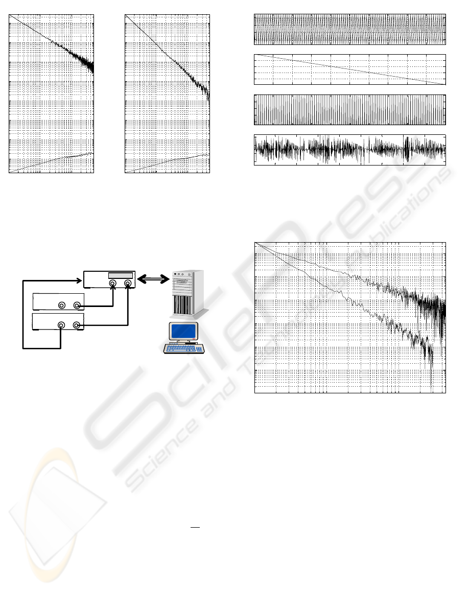
In many practical situations two or more noise
processes simultaneously affect clocks performance.
In this cases instability of the device under test is ex-
plained away through the behaviour of the upper en-
veloping curve. If the individual variance curves cross
each other, it is possible to see the slope changes in the
variance curve, for a time-series which includes sev-
eral types of noise(Vernotte, 1993). This situation is
shown in figures 7 and 8.
ICINCO 2005 - SIGNAL PROCESSING, SYSTEMS MODELING AND CONTROL
312

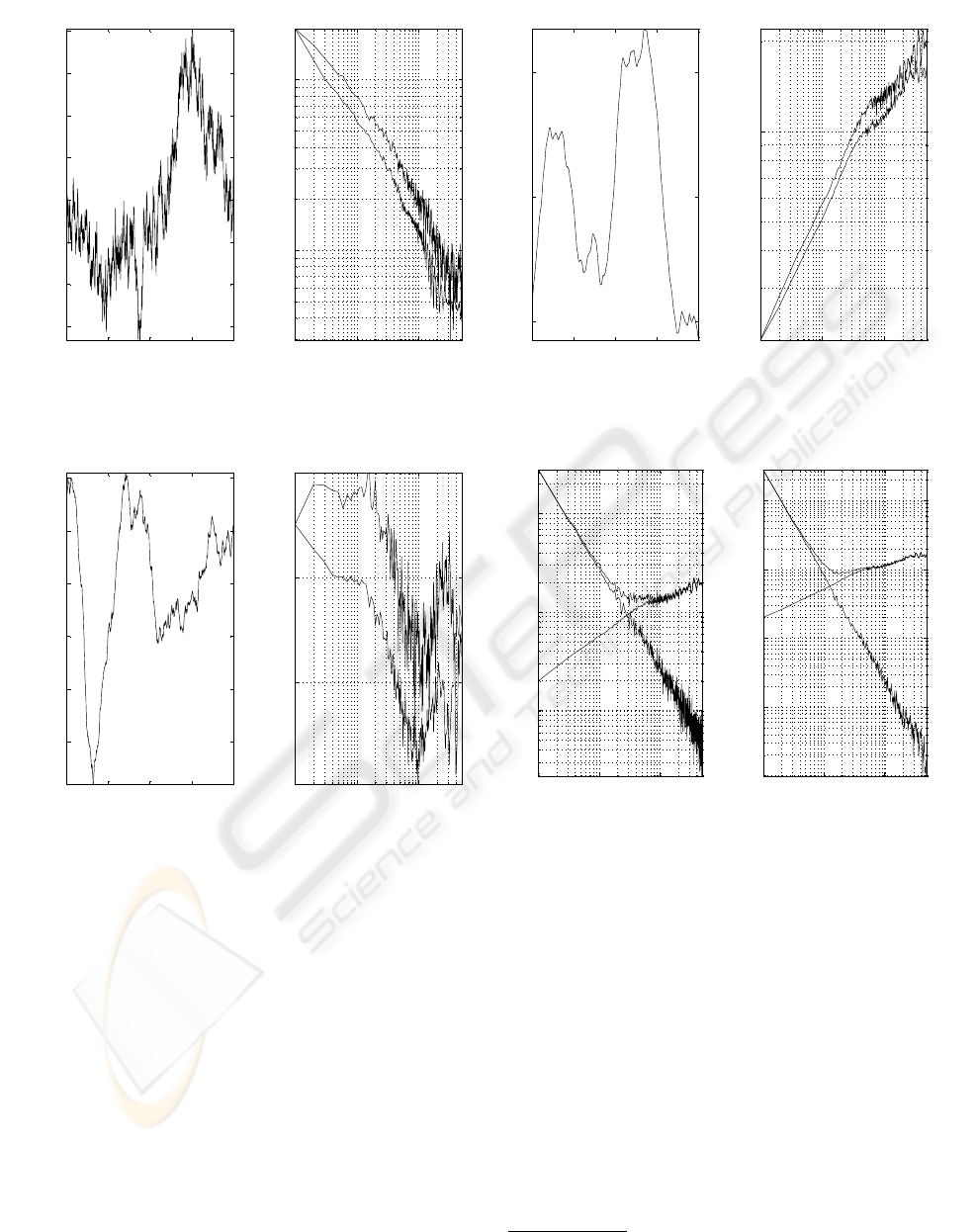
0.1 0.2 0.3 0.4
-6
-4
-2
0
2
4
6
8
x 10
-4
Time (s)
Amplitude (V)
White freq. mod.
10
-4
10
-3
10
-2
10
-2
10
-1
log(tau)
log(sigma)
AVAR and MVAR; beta=-2
Figure 4: Characterization of a noise process corresponding
to β = −2.
0.1 0.2 0.3 0.4
-3
-2
-1
0
1
2
x 10
-4
Time (s)
Amplitude (V)
Flicker freq. mod.
10
-4
10
-3
10
-2
10
-2.4
10
-2.3
10
-2.2
log(tau)
log(sigma)
AVAR and MVAR; beta=-3
Figure 5: Characterization of a noise process corresponding
to β = −3.
In figure 7, the individual variance curves cross. So
the enveloping curve characterizes the short-term in-
stability. By the contrary, in figure 8 the β = 0 noise
processes has a variance greater than the β = −4 per-
turbation. In this case the enveloping curve is the first
(upper) AVAR curve.
4 EXPERIMENTAL RESULTS
AND CONCLUSIONS
A high resolution function generator is chosen as de-
vice under test. It is set up to deliver a 1.1 Hz TTL
signal. The experimental arrangement is depicted in
0.1 0.2 0.3 0.4
-1
0
1
x 10
-4
Time (s)
Amplitude (V)
Random walk freq. mod.
10
-4
10
-3
10
-2
10
-3
log(tau)
log(sigma)
AVAR and MVAR; beta=-4
Figure 6: Characterization of a noise process corresponding
to β = −4.
10
-4
10
-3
10
-2
10
-4
10
-3
10
-2
log(tau)
log(sigma)
AVAR
10
-4
10
-3
10
-2
10
-6
10
-5
10
-4
10
-3
10
-2
log(tau)
MVAR
Figure 7: Noise processes corresponding to β = 0 and β =
−4. Situation of changing slope.
figure 9. The measurement system comprises a TIC
4
,
a GPS receiver and the frequency source under test.
These instruments have been connected via GPIB to
the computer. Data points are captured every 1 s.
Time interval counters (TICs) and GPS receivers
are widely used in traceable frequency calibrations.
A transfer standard receives a signal that has a cesium
oscillator as source (Lombardi, 1999). This signal de-
livers a cesium derived frequency to the user, who is
benefited as not all laboratories can afford a cesium
(Lombardi, 1996). These instruments differ in speci-
fications and details regarding the time base, the main
gate and the counting assembly. Furthermore, manu-
facturers tend to omit the conditions under these spec-
4
Time Interval Counter
A GRAPHICAL REVIEW OF NOISE-INSTABILITY CHARACTERIZATION IN ELECTRONIC SYSTEMS
313

10
-4
10
-3
10
-2
10
-3
10
-2
10
-1
10
0
10
1
10
2
10
3
10
4
log(tau)
log(sigma)
AVAR
10
-4
10
-3
10
-2
10
-3
10
-2
10
-1
10
0
10
1
10
2
10
3
10
4
log(tau)
log(sigma)
MVAR
Figure 8: Noise processes corresponding to β = 0 and β =
−4. The upper noise process is the enveloping curve.
ifications have been provided or measured.
GPIB
GPS Receiver
TIC
UTC 1 pps
CHA
CHB
10 MHz
Ext. Ref.
Input
oscil
lator
50
Ω
output
1.1 Hz
Figure 9: Experimental arrangement.
Figure 10 shows the signals involved in the mea-
surement process. Each measurement cycle corre-
sponds to 1 s. The bottom graph corresponds to
the instantaneous phase-deviation series, which com-
prises m = 898 data. These data are the result of fil-
tering the spiky time-series of phase differences, and
are used to perform the calibration. These data are
supposed to be corrupted by white noise, with a rec-
tangular probability density function. This is corrob-
orated later by means of AVAR and MVAR.
The ratio of the classical variance (VAR) to the Al-
lan variance (AVAR) provides a primary test for white
noise. This quantity (0.672) is less than 1 + 1/
√
m ≃
1.033; thus it is probably safe to assume that the data
set is dominated by white noise, and the classical sta-
tistical approach can safely be used. Failure of the
test does not necessarily indicate the presence of non-
white noise (Fluke, 1994).
A slope test (based in AVAR and MVAR curves)
has been developed to confirm the presence of white
noise. AVAR and MVAR curves are depicted in figure
11.
Measures of the slopes over the log-log graphs in
100 200 300 400 500 600 700 800 900 1000
0.2
0.4
0.6
0.8
From GPIB (sec.)
Signals in the measurement system
100 200 300 400 500 600 700 800 900 1000
-80
-60
-40
-20
0
Phase shift (sec.)
100 200 300 400 500 600 700 800 900
0.1
0.12
0.14
0.16
0.18
x(i) (sec.)
100 200 300 400 500 600 700 800
0.0906
0.0908
0.091
0.0912
Measurement cycles
Filtered x(i), (sec.)
Figure 10: Signals in the measurement chain. From top to
bottom: original data from the TIC and the GPIB interface,
accumulated phase shift, spiky phase differences, filtered
phase differences.
10
0
10
1
10
2
10
-9
10
-8
10
-7
10
-6
10
-5
10
-4
log(tau)
log(VAR), log(MVAR)
Figure 11: AVAR (upper) and MVAR (lower) log-log
curves. The final calibration period is τ = 500 × τ
0
for
τ
0
= 1 s.
figure 11 offer the results -1 and -1.5 for log(AV AR)
vs. log(τ), and log(M V AR) vs. log(τ), respec-
tively; which indicate that a white phase modulation
process is coupled to the frequency source under test
(see table 1).
ACKNOWLEDGEMENT
The authors would like to thank the Spanish Min-
istry of Education and Science for funding the project
DPI2003-00878 which involves noise processes mod-
elling and time-frequency calibration.
ICINCO 2005 - SIGNAL PROCESSING, SYSTEMS MODELING AND CONTROL
314

REFERENCES
Allan, D. (1987). Time and frequency (time-domain)
characterization, estimation, and prediction of preci-
sion clocks and oscillators. IEEE Transactions on
Ultrasonics, Ferroelectrics, and Frequency Control,
34(752):647–654.
Fluke (1994). Calibration: Philosophy in Practice. Fluke,
2 edition.
Greenhall, C. (1988). Frequency stability review. TDA
progress report. Technical Report 42-88, Communi-
cations Systems Research Section.
Howe, D., Allan, D., and Barnes, J. (1999). Properties of
oscillator signals and measurement methods. Tech-
nical report, Time and Frequency Division. National
Institute of Standards and Technnology.
IEEE (1988). IEEE standard definitions of physical quan-
tities for fundamental frequency and time metrology.
Technical Report IEEE Std 1139-1988, The Institute
of Electrical and Electronics Engineers, Inc., 345 East
47th Street, New York, 10017, USA.
Lesage, P. and Ayi, T. (1984). Characterisation or frequency
stability: Analysis of the modified allan variance and
properties of its estimate. IEEE Trans. on Instrumen-
tation and Measurement, IM-33(4):332–336.
Lombardi, M. (1996). An introduction to frequency calibra-
tions. The International Journal of Metrology, (Janu-
ary/February 1996).
Lombardi, M. (1999). Traceability in time and frequency
metrology. The International Journal of Metrology,
(September/October 1999).
Rutman, J. and Walls, F. (1991). Characterization of fre-
quency stability in precision frequency sources. Proc.
IEEE, 79(7):952–960.
Sullivan, D., Allan, D., Howe, D., and Walls, F. (1990).
Characterization of clocks and oscillators. NIST Tech
Note, 868(1337). BIN: 868.
Vernotte (1993). Oscillator noise analysis: Multivariance
measurement. IEEE Transactions on Instrumentation
and Measurement, 42(2):342–350.
Vig, J. R. (2001). A Tutorial For Frequency Control and
Timing Applications.
Wei, G. (1997). Estimations of frequency and its drift rate.
IEEE Trans. on Instrumentation and Measurement,
46(1):79–82.
A GRAPHICAL REVIEW OF NOISE-INSTABILITY CHARACTERIZATION IN ELECTRONIC SYSTEMS
315