APPLYING SIGNAL PROCESSING TECHNIQUES TO WATER

LEVEL ANOMALY DETECTION

Carl Steidley, Richard Rush, David Thomas, Phillipe Tissot, Alex Sadovski, Ray Bachnak

Texas A&M University Corpus Christi

Corpus Christi, TX 78412 5825

USA

Keywords: Environmental monitoring and control, Filtering, Change detection.

Abstract: The Texas Coastal Ocean Observation Network (TCOON) consists of more than 50 data gathering stations

located along the Texas Gulf coast from the Louisiana to Mexico borders. Data sampled at these stations

include: precise water levels, wind speed and direction, atmospheric and water temperatures, barometric

pressure, and water currents. The measurements collected at these stations are often used in legal

proceedings such as littoral boundary determinations; therefore data are collected according to National

Ocean Service standards. Some stations of TCOON collect parameters such as turbidity, salinity, and other

water quality parameters. All data are transmitted back to Texas A&M University Corpus Christi (A&M-

CC) at multiples of six minutes via line-of-sight packet radio, cellular phone, or GOES satellite, where they

are then processed and stored in a real-time, web-enabled database. TCOON has been in operation since

1988. This paper describes a software project based upon signal processing techniques to be utilized with

the TCOON meteorological database to detect spikes in water level. Water level readings are frequently

victim to abnormal water levels caused by ship wakes, affected equipment scrambled by thunder, or

corrupted by transmission errors. Since these water levels are the bases for a number of research

calculations, such as, oil-spill response, navigation safety, environmental research, and recreation, it is

essential to be able to make these water level data as correct and spike free as possible.

1 INTRODUCTION

The TCOON filter system consists of two

implementations of spike detection algorithms

which accept parameters from the TCOON

meteorological database or series of data and

return the location of spikes within the processed

series, since spikes represent inaccurate data it is

imperative to remove this data from our research

database (Krukowski 2000, Michaud, 2001). We

discuss these methods below and then provide a

comparison of results.

2 FINITE IMPULSE RESPONSE

METHOD

2.1 Theory

Digital filters can have an 'arbitrary response':

meaning, the attenuation is specified at certain

chosen frequencies, or for certain frequency bands.

These filters are also characterized by their

response to an impulse: a signal consisting of a

single value followed by zeroes. The impulse

response is an indication of how long the filter

takes to settle into a steady state: it is also an

indication of the filter's stability - an impulse

response that continues oscillating in the long term

indicates the filter may be prone to instability. The

impulse response defines the filter just as well as

does the frequency response. Output from a digital

filter is made up from previous inputs and previous

outputs, using the operation of convolution. As

indicated in the following equation, two

303

Steidley C., Rush R., Thomas D., Tissot P., Sadovski A. and Bachnak R. (2005).

APPLYING SIGNAL PROCESSING TECHNIQUES TO WATER LEVEL ANOMALY DETECTION.

In Proceedings of the Second International Conference on Informatics in Control, Automation and Robotics - Signal Processing, Systems Modeling and

Control, pages 303-309

DOI: 10.5220/0001152503030309

 SciTePress

convolutions are involved: one with the previous

inputs, and one with the previous outputs. In each

case the convolving function is called the filter

coefficients.

Since filtering is a frequency selective

process, the important thing about a digital filter is

its

frequency response. The filter's frequency response

can be calculated from its filter equation as

follows:

The frequency response H(f) is a continuous

function, even though the filter equation is a

discrete summation. While it is nice to be able to

calculate the frequency response given the filter

coefficients, when designing a digital filter we

want to do the inverse operation: that is, to

calculate the filter coefficients having first defined

the desired frequency response. So we are faced

with an inverse problem. Sadly, there is no general

inverse solution to the frequency response

equation. To make matters worse, we want to

impose an additional constraint on acceptable

solutions. Usually, we are designing digital filters

with the idea that they will be implemented on

some piece of hardware. This means we usually

want to design a filter that meets the requirement

but which requires the least possible amount of

computation: that is, using the smallest number of

coefficients. So we are faced with an insoluble

inverse problem, on which we

wish to impose

additional constraints. This is why digital filter

design is more an art than a science: the art of

finding an acceptable compromise between

conflicting constraints. If we have a powerful

computer and time to take a coffee break while the

filter calculates, the small number of coefficients

may not be important - but this is a pretty sloppy

way to work and would be more of an academic

exercise than a piece of engineering (Kuo, 2001).

It is much easier to approach

the problem of

calculating filter coefficients if we simplify the

filter equation so that we only have to deal with

previous inputs (that is, we exclude the possibility

feedback). The filter equation is then simplified

as follows:

If such a filter is subjected to an impulse (a

signal consisting of one value followed by zeroes)

then its output must necessarily become zero after

the impulse has run through the summation. So the

impulse response of such a filter must necessarily

be finite in duration. Such a filter is called a Finite

Impulse Response filter or FIR filter. The filter's

frequency response is also simplified, because all

the bottom half goes away, as indicated in the

following equation:

It so happens that this frequency response is

just the Fourier transform of the filter coefficients.

The inverse solution to a Fourier transform is well

known: it is simply the inverse Fourier transform.

So the coefficients for an FIR filter can be

calculated simply by taking the inverse Fourier

transform of the desired frequency response.

To avoid having many small coefficients, we

can truncate or discard the small valued

coefficients. Truncating the filter coefficients

means we have a truncated signal, and a truncated

signal has a broad frequency spectrum. So

truncating the filter coefficients means the filter's

frequency response can only be defined coarsely.

Luckily, there is a way to sharpen up the frequency

spectrum of a truncated signal, by applying a

window function. So after truncation, we can apply

a window function to sharpen up the filter's

frequency response. This provides us with an even

better algorithm for calculating FIR filter

coefficients, the so-called window method of filter

design.

FIR filter coefficients can be calculated using

the window method:

• pretend we don't mind lots of filter

coefficients

• specify the desired frequency response

using lots of samples

• calculate the inverse Fourier transform

• this gives us a lot of filter coefficients

• so truncate the filter coefficients to give

us less

Output

Previous input previous output

Y[n] = ∑ c[k] * x[n-k] + ∑ d[j] * y[n-j] (1)

∑ c[k] * exp(-2Πjk(f∆))

H(f) = ------------------------- (2)

1 - ∑ d[j] * exp(-2Πjk(f∆))

Y[n] = ∑ c[k] * x[n-k] (3)

∑ c[k] * exp(-2Πjk(f∆))

H(f) = ------------------------- (4)

1 - ∑ d[j] * exp(-2Πjk(f∆))

ICINCO 2005 - SIGNAL PROCESSING, SYSTEMS MODELING AND CONTROL

304

• apply a window function to sharpen up

the filter's frequency response

• then calculate the Fourier transform of the

truncated set of coefficients to see if it

still matches our requirement

However, no matter how many filter

coefficients you throw at it, you cannot improve on

a fixed window's attenuation. This means that the

art of FIR filter design by the window method lies

in an appropriate choice of window function. For

example, if you need an attenuation of 20 dB or

less, then a rectangle window is acceptable. If you

need 43 dB you are forced to choose the Hamming

window, and so on. Sadly,

the better window

functions need more filter coefficients before their

shape can be adequately defined. So if you need

only 25 dB of attenuation you should choose a

triangle window function which will give you this

attenuation: the Hamming window, a form of

generalized cosine window, for example, would

give you more attenuation but require more filter

coefficients to be adequately defined - and so

would be wasteful of computer power.

The art of FIR filter design by the window method

lies in choosing the window function which meets

your requirement with the minimum number of

filter coefficients. You may notice that if you want

an attenuation of 30 dB you are in trouble: the

triangle window is not good enough but the

Hamming window is too good (and so uses more

coefficients than you need). The Kaiser window

function is unique in that its shape is variable. A

variable parameter defines the shape, so the Kaiser

window ,described mathematically below, is

unique in being able to match precisely the

attenuation you require without overperforming.

FIR filter coefficients can be calculated using

the window method. But the window method does

not correspond to any known form of optimization.

In fact it can be shown that the window method is

not optimal - by which we mean, it does not

produce the lowest possible number of filter

coefficients that just meets the requirement. The

art of FIR filter design by the window method lies

in choosing the window function which meets your

requirement with the minimum number of filter

coefficients. If the window method design is not

good enough we have two choices:

• use another window function and try

again

• do something clever

The Remez Exchange algorithm is something

clever. It uses a mathematical optimization

method. Thus, using the Remez Exchange

algorithm to design a filter we might proceed

manually as follows:

• choose a window function that we think

will do

• calculate the filter coefficients

• check the actual filter's frequency

response against the design goal

• if it overperforms, reduce the number of

filter coefficients or relax the window

function design

• try again until we find the filter with the

lowest number of filter coefficients

possible

In a way, this is what the Remez Exchange

algorithm does automatically. It iterates between

the filter coefficients and the actual frequency

response until it finds the filter that just meets the

specification with the lowest possible number of

filter coefficients. Actually, the Remez Exchange

algorithm never really calculates the frequency

response: but it does keep comparing the actual

with the design goal.

The Remez method produces a filter which

just meets the specification without

overperforming. Many of the window method

designs actually perform better as you move

further away from the passband: this is wasted

performance, and means they are using more filter

coefficients than they need. Similarly, many of the

window method designs actually perform better

than the specification within the passband: this is

also wasted performance, and means they are using

more filter coefficients than they need. The Remez

method performs just as well as the specification

but no better: one might say it produces the worst

possible design that just meets the specification at

the lowest possible cost (Proakis, 2003).

[i] = 0.54 – 0.46 cos(2∏i / M) (5)

The Hamming window. These windows run from i =

0 to M, for a total of M+1 points.

_________

(Πα√1 – (2k/n-1)

) if 0≤k≤n (6)

(Πα)

0 otherwise

APPLYING SIGNAL PROCESSING TECHNIQUES TO WATER LEVEL ANOMALY DETECTION

305

2.2 Applying The Theory To

TCOON Database Data

TCOON data is recorded with a frequency of one

value every six minutes (or 0.00278 values a

second), so 10 consecutive values equal one hour’s

worth of data. Utilizing a filter design software

system which is an implementation of the Remez

Exchange Algorithm we determined a set of

coefficients to operate over 10 consecutive data

points that occur every six minutes (a frequency of

0.00278 Hz), that is, one hour of TCOON water

level data (

Sadovski, 2004, Bowles, 2004, Sadovski,

2003, Steidley, 2004) .

These coefficients are multiplied against a

sliding window applied to the data series. The

result of the filter for a given value is the sum of

the current value times the first coefficient, plus

the value before the current value times the second

coefficient, plus the value before the current value

times the second coefficient, plus the value two

values before the current value times the third

coefficient, etc. until all ten coefficients have been

used (See Figure 1).

Since the filter requires nine preceding values

to calculate the filtered equivalent for a value, the

first nine values in a series cannot be processed

and are “lost” in terms of the resulting series. That

is, this process applies a phase shift to the data

series. So, the entire filtered data series is reversed

and run through the FIR filter a second time, with

the coefficients, in response to this phase shift.

Because each pass through the filter discards the

first nine values in a series, the original data series

loses nine values at both ends. This means that to

have at least a single value in the result of the two

passes through the filter, a minimum of 19 values,

or one hour and fifty four minutes’ worth of data

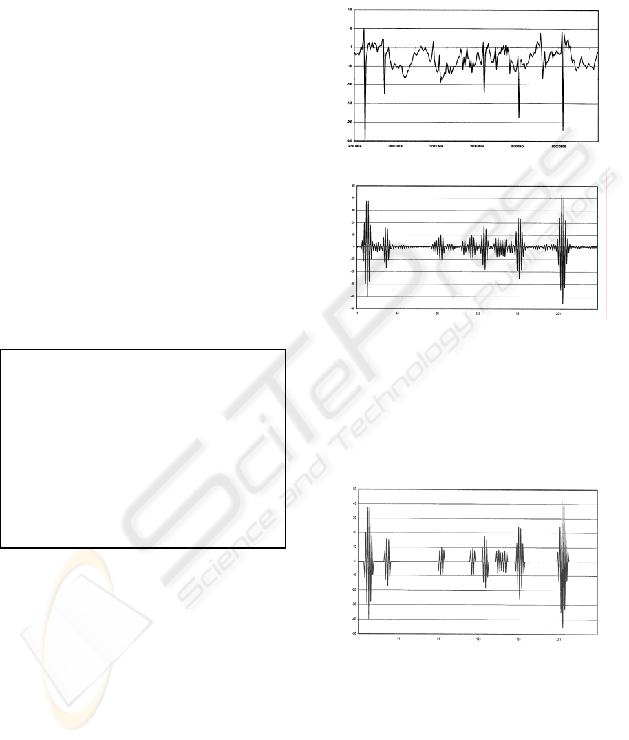
must be provided. After processing raw data

(Figure 2) through the FIR filter twice, data that

behaves normally with respect to preceeding data,

is minimized, whereas abnormally behaving data

(Figure 3) remains significant.

Figure 2: Primary Water Level Data

Figure 3: Filtered Data

To remove the data that cannot be spikes from

the output of filter we compute the root mean

square value of the filtered data and discard all

values that are less than or equal to the RMS value

(Figure 4). The data point with the greatest

absolute value in each group is labeled a spike

(Figure 5).

Figure 4: Significant Filtered Values

result = FIR(series)

result = FIR(reverse result)

rms = RMS(result)

for each in result

if result{current] is <= rms

result[current] = 0

if result[current] == 0 and result[spike] != 0

push spikes, spike

spike = 0

if result[current] is > result[spike]

spike = current

return spikes

Figure 1: Finite Impulse Response Filter Psuedocode

ICINCO 2005 - SIGNAL PROCESSING, SYSTEMS MODELING AND CONTROL

306

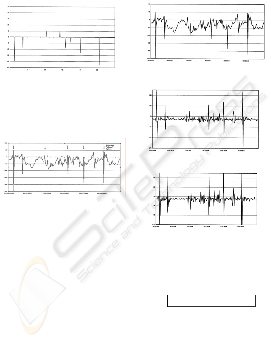
Figure 5: Greatest Filtered Values

Since we are detecting only the greatest value

in each group of potential spikes, two consecutive

spikes, one spike that is long enough to appear in

two data acquisition values, or a separate and

smaller spike that occurs within the shadow of a

larger spike can escape detection (Figure 6).

Figure 6: Primary Water Level Data Including Spikes

and Potentially “Missed” Spikes

3 DIFFERENCE EXAMINATION

METHOD

The difference examination method is dependant

upon the second difference of the data series. As

the difference between two points represents the

change between those two points over one

increment of time (six minutes in the case of this

data), the second difference represents the change

between changes. The algorithm for this method

first builds a series out of the differences between

the original series’ values and then builds a third

series from the differences between the values in

the second constructed series (Figures 7, 8, 9).

Figure 7: Primary Water Level

Figure 8: First Differences

Figure 9 Second Differences

After computing the second differences of the

original data series, the root mean square of the

second difference is computed. Any value greater

than twice the root mean square of the second

difference is labeled a spike (Figure 10).

RMS

diff

= RMS

+ RMS

(7)

APPLYING SIGNAL PROCESSING TECHNIQUES TO WATER LEVEL ANOMALY DETECTION

307

Figure 10: Second Differences Greater than Twice the

Root Mean Square

4 COMPARISON OF THE TWO

SPIKE DETECTION

METHODS

To determine the presence of spikes within a data

set generally requires the use of some subjective

evaluation procedure, we choose to present the

data visually in the form of graphs. Further, since

the determination of spikes in actual recorded data

is difficult at best, we chose to evaluate and

compare the two spike detection methods on

simulated data. We created software

which

generates spike data psuedorandomly. We can,

therefore, execute both methods on a data series

simulating the same time and place repreatedly, the

combined results of which can be used to generate

some basic statistics.

In our tests, both detection methods were

applied to forty different series of data generated

by our spike simulator. Each data series had one

percent of its data converted to spikes. Table 1

illustrates the results of the execution.

5 DISCUSSION

The spikes between 25 and 34 cm are the largest

spikes applied to the data and are, therefore, the

most important spikes to detect. Spikes between

15 and 24 cm are desirable to detect, while spikes

between 5 and 14 cm are negligible and are the

least important to locate. A low number of data

points incorrectly identified as spikes is important,

since data points identified as spikes will be

removed from the TCOON database. Too many

values incorrectly identified will corrupt the use

and value of the TCOON database.

Table 1: Mean Average Spike Detection Results

FIR DIFF FIR % DIFF %

Number of

Data Points

7440 7440 - -

Number of

Spikes

Found

70.35 172.03 - -

25 cm to 34

cm Spikes

found

23.00 24.52 93.08 99.46

25 cm to 34

cm Spikes

missed

1.65 0.12 6.92 0.54

15 cm to 24

cm Spikes

found

22.57 24.38 90.40 97.45

15 cm to 24

cm Spikes

missed

2.42 0.62 9.60 2.55

5 cm to 14

cm Spikes

found

20.35 3.73 81.95 14.55

5 cm to 14

cm Spikes

missed

4.58 21.20 18.05 85.45

Incorrectly

identified

spikes

4.42 119.40 6.30 69.42

5.1 Finite Impulse Response

Method

The results depicted in Table 1 indicate that the

Finite Impulse Response Method behaves fairly

well. Although an average of 93.08% of the major

spikes were found, it is likely that many of the

major spikes that were missed were hidden by

proximity to other, larger spikes. Repeated

applications of this method to the same data series,

with detected data spikes removed, will

cumulatively improve its performance. Similarly,

this method performed well, but not excellently,

when detecting smaller spikes (those between 5

and 24 cm), performance that is likely to

cumulatively improve over repeated applications.

The number of data spikes incorrectly identified as

spikes was low: 6.3% of the spikes it found were

not spikes; and average of 4.42 incorrect spikes

were found in an entire month’s worth of data

(Bowles, 2004).

5.2 Difference Examination

Method

As indicated in Table 1, the Difference

Examination Method does not perform as well as

the FIR method. This method found nearly all of

ICINCO 2005 - SIGNAL PROCESSING, SYSTEMS MODELING AND CONTROL

308

the major (99.46%) spikes and significant

(97.45%) spikes. It missed a large majority

(85.45%) of the small spikes. This method

detected nearly 7% more spikes 15 cm or greater

that the FIR method. However, this method falters

severely in its error rate. 70% of the spikes

detected by this method were incorrect. Although

this would result in only 1.6% of the data set being

falsely identified as a spike, we feel this is a

dangerously high error rate.

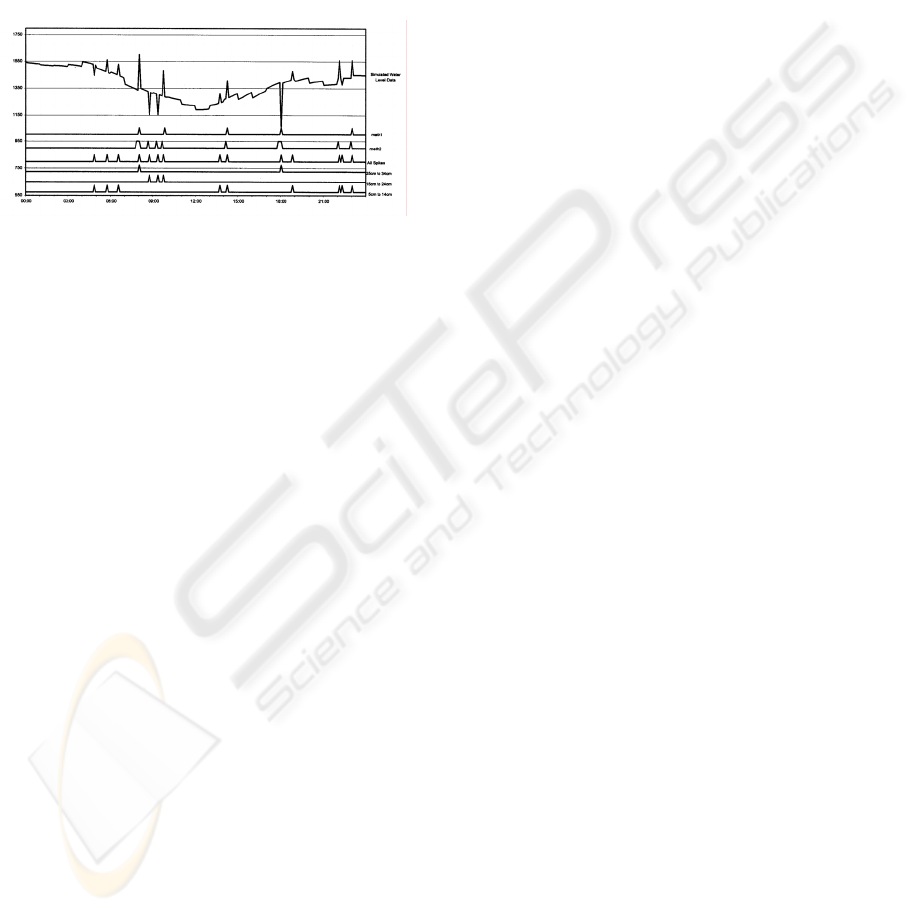
Figure 11: Simulated Water Level Data for 24 Hour

Period

6 CONCLUSIONS

Two different software methods for detecting

spikes in water level data have been implemented.

The first of these makes use of a finite impulse

response filter. A data series is passed through the

filter forwards, then backwards; this process

minimizes values within the series that appear

normal with respect to the previous hour’s values

while exacerbating values that are not similar to

the previous hour’s values. The remaining

significant values are then examined and the

largest value within each set of contiguous

significant values is labeled as a spike. The second

method deals with second differences of the data

series being examined. In this method, values that

are significantly larger than the second derivative

of the recorded data is labeled a spike. For our

purposes the FIR method outperforms the second

differences method.

ACKNOWLEDGEMENT

This project is partially supported by National

Aeronautics and Space Administration grant

NCC5-517.

REFERENCES

Artur Krukowski, Izzet Kale: DSP System Design:

Complexity Reduced Iir Filter Implementation for

Practical Applications, Kluwer Academic

Publishers, 2000.

Michaud, P., R.S. Dannelly, and G. Jeffress, C. Steidley,

“Real-Time Data Collection and the Texas Coastal

Ocean Observation Network”, Proceedings of the

Emerging Technologies Conference of the

Instrumentation, Systems, and Automation

Conference, CD-ROM Session ETCON19,

September 2001.

Sen M. Kuo, Woon-Seng Gan: Digital Signal

Processors: Architectures, Implementations, and

Applications, Prentice Hall, 2001.

John Proakis, Dimitris Manolakis: Digital Signal

Processing - Principles, Algorithms and

Applications, Pearson, 2003.

Sadovski, Alexey, Carl Steidley, Aimee Mostella,

Phillipe Tissot, “Intergration of Regression and

Harmonic Analysis to Predict Water Levels in

Estuaries and Shallow Water of the Gulf of Mexico,”

WSEAS Transactions on Systems, pp. 2686-2693,

Vol. 3, Issue 8, October 2004.

Bowles, Zack, Alexey Sadovski,Phillipe Tissot, Scott

Duff, Patrick Michaud, Carl Steidley, "Engineered

training sets: enhancing the learning power of

artificial neural networks for water level forecasts",

Proceedings of XIV International Symposium on

Mathematical Methods Applied to the Sciences, pp

30-31, San Jose, Costa Rica, February 2004.

Sadovski, Alexey L., Phillipe Tissot, Gary Jeffress, Carl

Steidley, "Neural Network and Statistics-Based

Systems for Predictions in Coastal Studies",

Intelligent Engineering Systems Through Artificial

Neural Networks, Volume 1, 3, pp 689-694, ASME

Press, New York, 2003.

Steidley, C., A. Sadovsky, R. Bachnak, and K. Torres,

“Modeling Methods for Coastal Environmental

Studies,” Proc. 19th International Conference on

Computer Applications and Their Applications

(CATA 2004), pp. 59-64, March18-20, 2004,

Seattle, WA.

APPLYING SIGNAL PROCESSING TECHNIQUES TO WATER LEVEL ANOMALY DETECTION

309