Pattern recognition algorithms for polyphonic

music transcription

Antonio Pertusa and Jos´eM.I˜nesta

Departamento de Lenguajes y Sistemas Inform´aticos

Universidad de Alicante, Spain

Abstract. The main area of work in computer music related to informa-

tion systems is known as music information retrieval (MIR). Databases

containing musical information can be classiﬁed into two main groups:

those containing audio data (digitized music) and those that ﬁle sym-

bolic data (digital music scores). The latter are much more abstract that

the former ones and contain a lot of information already coded in terms

of musical symbols, thus MIR algorithms are easier and more eﬃcient

when dealing with symbolic databases. The automatic extraction of the

notes in a digital musical signal (automatic music transcription) permits

applying symbolic processing algorithms to audio data. In this work we

analize the performance of a neural approach and a well known non

parametric algorithm, like nearest neighbours, when dealing with this

problem using spectral pattern identiﬁcation.

1 Introduction

Music transcription is deﬁned as the act of listening to a piece of music and writ-

ing down music notation for the notes that make up the piece [1]. The automatic

transcription of monophonic signals (only one note playing simultaneously) is a

largely studied problem. Several algorithms have been proposed that are reli-

able, commercially applicable, and operate in real time. Nevertheless, automatic

polyphonic music transcription is an open research problem, because not even

the perceptual mechanisms involved in the isolation of diﬀerent notes and instru-

ments and their insertion in the corresponding musical phrases are clear. This

fact causes a lack of computational models to emulate these processes.

The availability of robust and reliable algorithms to solve this task has an

important application in music information retrieval (MIR) because digital au-

dio databases could be analysed and indexed in terms of symbolic data, much

more abstract and musically informative. Recent state-of-the-art in music tran-

scription has been discussed by Klapuri [2].

The methods discussed in this paper are in the frequency domain [3], like

those that analyse the sound spectrogram in search for clues about the notes that

originated that sound. Here, we try to apply two very diﬀerent approaches in

pattern recognition, like dynamic neural networks and a non parametric method,

Pertusa A. and M. Iñesta J. (2004).

Pattern recognition algorithms for polyphonic music transcription.

In Proceedings of the 4th International Workshop on Pattern Recognition in Information Systems, pages 80-89

DOI: 10.5220/0002681000800089

 SciTePress

like nearest neighbours. Connectionist approaches have been used in music tran-

scription [4], mainly with piano music [5], and they seem to be a good tool for

building transcription systems. We will also try to ﬁnd out whether a simple

nearest neighbour classiﬁer is able to perform similarly, or on the other hand,

neural learning provides unique features to solve this diﬃcult problem.

2 Methodology

The spectral pattern of a given sound signal, s(t), is the energy distribution that

can be found in the constituent partial frequencies of its spectrum, S(f). This

pattern is the most important parameter for characterising the musical timbre.

In this work, the music transcription problem is posed through the identiﬁcation

of the spectral pattern of the instrument, using two very diﬀerent pattern recog-

nition algorithms: on one hand a connectionist dynamic algorithm like time-delay

neural networks (TDNN) [6] and, on the other hand, a geometric non supervised

algorithm like k-nearest neighbours (k-NN). Both algorithms will use as train-

ing set spectrograms computed from polyphonic melodies played by a target

instrument (monotimbric melodies).

To achieve this goal, we need to build input and output pairs formed by the

spectra of the sound produced by a source

for diﬀerent times around a given

instant t

. Input is {S(f,t

i+j

)} for j ∈ [−m, +n] for each frequency f ,beingm

and n the number of windows considered before and after the central time, t

Output consists of a coding of the set of possible notes ν(t

) that are active at

that moment in order to produce those spectra.

After learning the spectral pattern, it is expected that a pattern recognition

algorithm will be able to detect the notes in a digitization of a new melody

produced by that sound source from the detection of occurrences of that pattern.

2.1 Construction of the input-output pairs

The training set has to be formed by pairs {{S(f,t

i+j

),j ∈ [−m, +n]}, ν(t

)}.

We need to have a set of music scores and synthesize sounds according to the

instructions in them in such a way that the correspondence between the spectrum

and the set of notes that have motivated it is kept at every moment. For this,

we have used MIDI ﬁles [7] and a software synthesizer developed by the Media

Lab at MIT named Csound [8].

First we will get into the details of the input data construction and then we

will describe the training outputs.

Input data. From the MIDI sequence, the digital audio ﬁle is synthesized and

the short-time Fourier transform (STFT) is computed, providing its spectrogram

We will only consider tuned sound sources, those that produce a musical pitch,

leaving apart those produced by random noise or highly inharmonic sources.

S(f,t). The STFT has been computed used a Hanning window, described at a

given instant τ by this expression:

w(τ)=



1 − cos

2πτ



where N = 2048 if the number of samples in the window. Also an overlapping

percentage of S = 50% has been applied in order to keep the spectral information

at both ends of the window. The original sampling rate was f

=44, 100 Hz, but

we have used an operational sampling rate of 44, 100/2=22, 050 Hz in order to

have less frequency bands. With these data, the time resolution for the spectral

analysis, ∆t = t

i+1

− t

, can be calculated as

∆t =

100f

=46.4 milliseconds .

The STFT provides 1024 frequency amplitudes between 0 and 11,025 Hz,

with a resolution of 10.77 Hz. For our analysis we will transform the spectrum

frequencies into bands in a logarithmic scale of a twelfth of octave (a semitone)

considering bands beginning in frequencies ranging from 50 Hz (a pitch close to

– G sharp of octave 0 – ) to 10,600 Hz (F

in pitch), almost eight octaves.

This way, we obtain b = 94 spectral bands that correspond to the 94 notes in

that range and they will be the input of our classiﬁers.

S(f, t=τ)

-96 dB --

0 dB --

θ --

50 Hz 11025 Hz

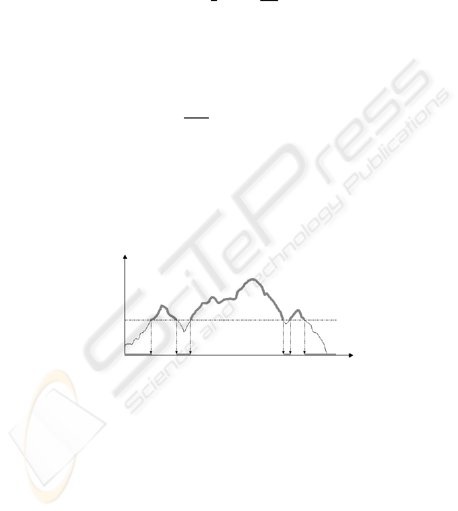
Fig. 1. Foreachspectrumalowlevelthresholdisappliedtoremovenoise.Then,the

amplitudes are normalized.

The amplitudes in the spectra are obtained in dB as attenuations from the

maximum amplitude. The dynamic range is normalized to the interval [−1, +1],

being the −1 value assigned to the maximum attenuation (−96 dB) and +1

assigned to the attenuation of 0 dB. In order to remove noise and emphasize

the important components in each spectrum, a low level threshold, θ, empiri-

cally established in −45 dB, is applied in such a way that if S(f

) <θthen

S(f

)=−1. See Fig. 1 for a picture of this scheme.

Usually, a note onset is not centered in the STFT window, so the bell-shape

of the Hanning window aﬀects the amplitude if the note starts at this position

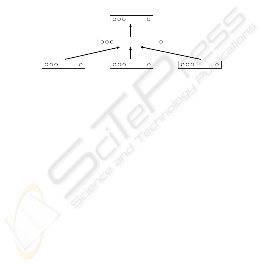
and some important amount of energy is lost. To solve this problem, the TDNN

uses a number of spectra in adjacent positions providing dynamical information

to the net. For each window position considered, 94 new input units are added

to the net, so the total number of input neurons will be b × (n + m +1). See

Fig. 2 for a scheme of this architecture.

..... ..... .....

................

.....

h(t )

ν( j , t ) ; j = 0, ... , b

S(f , t )

j = 0, ... , b

i-mj

S(f , t )

j = 0, ... , b

i+nj

S(f , t )

j = 0, ... , b

..... .....

Fig. 2. Network architecture and data supplied during training.

The upper limit for this context is conditioned by the fact that it is non sense

to have a number of windows so large that spectra from diﬀerent note subsets

appear frequently together at the input, causing confusion both in training and

recognition. Moreover, the computational cost depends on this number. A good

contextual information is desirable but not too much.

For the k-NN, the same can be done, giving a dimension of the vector space

of b × (n + m + 1), using the number spectra considered for the input context.

Output data. The notes sounding at each time, t

, are coded as a binary vector

of 94 components, ν(t

), in such a way that a value of ν(j, t

) = 1 for a particular

position j means that the j-th note is active at that time and 0 means that the

note is not active. The series of vectors ν(t),t =1, 2, ... will be named a binary

digital piano-roll (BDP). A brief example can be observed in Fig. 3.

The BDP is computed from the MIDI ﬁle, according to the notes that are

active at the times where the windows of the STFT are centered.

For the net, the output layer is composed of 94 neurons (see Fig. 2), one by

each possible note that can be detected. The vectors at each moment are the

training outputs shown to the net during the training phase, while the corre-

sponding spectra are presented to the input. During recognition, the output val-

ues for the neurons, y(j, t) ∈ [−1, +1], are compared with an activation threshold

(α) and a note is considered to be active if y(j, t

) >αand inactive otherwise.

This value controls the sensitivity of the net. There are other parameters free

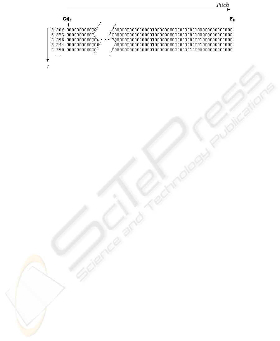
Fig. 3. Binary digital piano-roll coding the note activations (1’s) at each moment when

the spectrogram is computed. Each row represents the activations of the notes at a given

time.

for the net related to the training, like weight initialization, number of hidden

neurons, initial learning rate, etc. have shown to be less important.

Diﬀerent experimental results have been carried out varying these parameters

and the results presented below are those obtained by the best net in each case.

After some initial tests, a number of hidden neurons of 100 has proven to be a

good choice for that parameter, so the experiments have been obtained with this

number of hidden neurons.

For the k-NN, the vectors ν(t

) are associated as labels to the prototype

vectors in such a way that each prototype, that represents spectral values, has

the notes that produced that sound as a label. During recognition, the values of

the labels are summed by columns (notes), giving the number of notes found in

the k-neighbouring of the target spectrum. As in the case of the net, an activation

threshold is established as a fraction of k and only the notes found in a number

higher than it in the neighbouring are considered active.

2.2 Success assessment

A measure of the quality of the performance is needed. We will assess that quality

at two diﬀerent levels: 1) considering the detections at each window position

of the spectrogram in order to know what happens with the detection at

every moment. The output at this level will be named “event detection”; and 2)

considering notes as series of consecutive detections or missings along time.

At each time t

, the output activations, y(t

) (either neuron activations or

notes found in the neighbouring), are compared with the vector ν (t

). A suc-

cessful detection occurs when y(j, t

)=ν(j, t

)=1foragivenoutputposition

k. A false positive is produced when y(j, t

)=1andν(j, t

)=0(somethinghas

been wrongly detected), and a false negative is produced when y(j, t

)=0and

ν(j, t

) = 1 (something has been missed). These events are counted over an ex-

periment, and the sums of successes Σ

, false positives Σ

, and false negatives

−

are computed. Using all these quantities, the success rate in percentage for

detection is deﬁned as:

σ =

100Σ

+ Σ

−

+ Σ

With respect to notes, we have studied the output produced according to

the criteria described above and the sequences of event detections have been

analysed in such a way that a false positive note is detected when a series of

false positive events is found surrounded by silences. A false negative note is

deﬁned as a sequence of false negative events surrounded by silences, and any

other sequence of consecutive events (without silences inside) is considered as a

successfully detected note. The same equation as above is utilized to quantify

the note detection success.

3Results

A number of diﬀerent polyphonic melodies have been used, containing chords,

solos, scales, silences, etc. trying to have diﬀerent number of notes sounding

at diﬀerent times, in order to have enough variety of situations in the training

set. All notes are played with the same dynamics and noiseless. The number of

spectrum samples was 31,680.

In order to test the ability of the algorithms with waves of diﬀerent spectral

complexity, a number of experiments have been carried out for diﬀerent waves:

synthetic ones (sinusoidal and sawtooth waveforms) and synthezised sounds imi-

tating real instruments like a clarinet, using a physical modelling algorithm. Our

aim is to obtain results with complex waves of sounds close to real instruments.

The limitations for acoustical acquisition of real data and the need of an exact

timing of the emitted notes have conditioned our decision for constructing these

sounds using virtual synthesis models.

3.1 Parameter tuning

According to the size of the input context, the best results were obtained, both

for TDNN and k-NN, with one previous spectrogram window and zero posterior

windows. Anyway, these results have not been much better than those obtained

with one window at each side, or even 2+1 or 1+2. The detection was consistently

worse with 2+2 contexts and larger ones. It was also interesting to observe that

the success rate was clearly worse when no context was considered (around 20%

less than with the other non-zero contexts tested).

In order to test the inﬂuence of the activation threshold, α, some values have

been tested. High values cause a lot of small good activations to be missed and

a lot of false negatives appear. As the value of α gets low the sensibility and

precision of the output increases.

For the net, values α ∈ [−0.8, −0.7] have shown to be the best, and for the

k-NN, values of a fraction of k/2and2k/3 have provided the best performance,

but this is very sensitive to the value of k, because when k becomes large (we

have tested k ∈ [20, 1000]), the algorithm works better with small fractions,

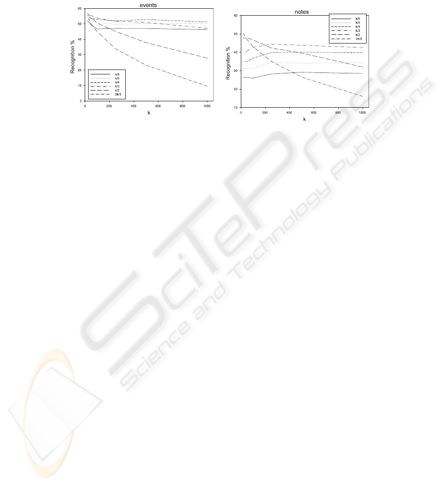
probably due to the limited size of the training set. See Fig. 4 for a picture of

this behaviour.

Fig. 4. Evolution of the detection rate for the clarinet with k-NN with diﬀerent values

of k and the threshold, α. (left) rates for events, (right) rates for notes.

Once these parameters have been tuned and their consistency for diﬀerent

waveshapes tested (within a small range of variation), we have performed a

number of cross-validation experiments in order to assess the performance with

the diﬀerent timbres. For this, each data set has been divided into four parts

and four sub-experiments have been made with 3/4 of the set for training and

1/4 for test. The presented results are those obtained by averaging the 4 sub-

experiments carried out on each data set.

3.2 Performance rates

As expected, the sinusoidal waves provided the best results using the nets (around

96% for events and 98% for notes), and were clearly worse for the k-NN.These

results were slightly worse using TDNN (around 91% for events and notes) when

applied to the sawtooth and the clarinet waveshapes, although they kept in good

ﬁgures. It seems that k-NN is not much sensitive to the complexity of the wave-

shape. In fact, it performed better when the spectra of the waveshapes were

more complex. All these ﬁgures are summarized in table 1.

These numbers are pointing to the fact that the TDNN is learning the spec-

tral pattern of each waveshape and then tries to ﬁnd it in complex mixtures

during the recognition stage. Thus, the more complex the pattern is, the harder

the recognition stage will be, and so, the performance will be poorer. On the

contrary, k-NN, is just exploring the training set looking for similarities and, for

this, the complexity of the pattern is not a key point.

For the TDNN, the event detection errors occurred in the onsets and oﬀsets

of the notes and most of the errors in note detection were missing notes of less

sine sawtooth clarinet

σ (%) TDNN ; k-NN TDNN ; k-NN TDNN ; k-NN

events 93.6 ; 50.4 92.1 ; 56.9 92.2 ; 56.9

notes 95.0 ; 42.8 91.7 ; 48.6 91.7 ; 50.3

Tabl e 1. Detection results in percentages obtained for the best classiﬁer en each case.

First row displays the event detection rates and the second one the note detection

rates.

than 0.1 s of duration (just one or two events). If these very short notes were

removed, almost a 100% of success was obtained with the net.

Note errors concentrated in very low-pitched notes, where the spectrogram is

computed with less precision and for very high notes, where the higher partials

in the note spectrum are cut oﬀ by the Nyquist frequency, or, even worse, folded

into the useful range, distorting the actual data, due to the aliasing eﬀect caused

by cutting down the sampling rate by a factor of two.

We have also tried to use a test set produced with a waveshape diﬀerent

from that used for the training set. The success rate has worsen (around 30%

lower in average) when a net trained with a given waveshape has been tested with

spectrograms of diﬀerent timbres, showing the high specialization of the training.

Probably, increasing the size and variety of the training set could improve this

particular point.

These ﬁrst results with real timbres suggest that the TDNN methodology can

be applied to other real instruments at least in the wind family, characterized by

being very stable in time. This makes the spectral pattern identiﬁcation easier

than in other more evolutive timbres like, for example, percussive instruments

as piano or vibes.

3.3 Evolution in time for note detection

Once the better performance of the neural approach has been tested, we show

a graphical study of the TDNN output, in order to analyse the kind of errors

produced. A new melody played with the clarinet timbre and not contained

neither in the training set nor in the test set was provided to the net and the

output displayed in ﬁgure 5 was obtained. The plot at the bottom side of the

ﬁgure is a comparative between the output of the net and the desired output. As

observed, the output of the net is very close to the original piano-roll. For this

melody, the event detection rate was 94.3 %, the proportion of false positives to

the number of events detected was 2.3 % and for false negatives was 3.4 %. For

notes, all of them were detected and just 3 short false positive notes appeared.

As it is observed, most of the event errors were produced in the transitions

between silence and sound or vice versa for some notes, due to the time resolution

and the excess of energy in a lapse were a note is not coded as sounding in the

BDP or the lack of energy where it is already sounding, according to the BDP.

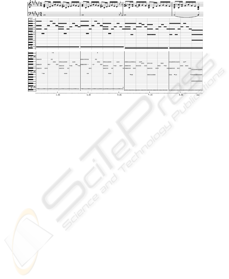
Fig. 5. Evolution in time of the note detection with the neural network for a new

melody using the clarinet timbre. Top: the original score; center: the melody as dis-

played in a sequencer piano-roll; down: the piano-roll obtained from the net output

compared to the original piano-roll. Notation: ‘o’: successfully detected events, ‘+’:

false positives, and ‘-’: false negatives.

For this sequence, only one note was really missed out and just six activations

corresponded to two non-existing notes.

4 Discussion and conclusions

This work has tested the feasibility of an approach based on pattern recognition

algorithms for polyphonic monotimbric music transcription. We have applied two

very diﬀerent approaches like time-delay neural networks (TDNN) and k-nearest

neighbours (k-NN) to the analysis of the spectrogram of polyphonic melodies of

synthetic timbres generated from MIDI ﬁles using a physical modelling virtual

syntheziser. All the notes in these melodies have been played with the same

dynamics and noiseless.

The TDNN have performed far better than the k-NN, reaching a detection

success of about 95% in average against about 50% in average for the k-NN.

The k-NN is unable to generalize and all its outputs are combinations of notes

already existing in the training set, whereas the TDNN is able to transcribe

note combinations in the training set never seen before. This fact suggests that

the network is able to learn the spectral pattern of a given waveshape and then

identify it when is found in the complex mixtures provided by the chords. An-

other point in this direction is that the performance of the net gets worse when

the spectral pattern of the waveshape is more complex, whereas spectral pattern

complexity and performance are not clearly correlated when using k-NN. These

results support the learning hypothesis for the nets.

Event detection errors are concentrated in the transitions, at both ends of the

note activations. This fact also conditions the detection of very short notes, one

or two events long. This kind of situations can be solved by a post-processing

stage over the net outputs along time. In a music score not every moment is

equally probable. The onsets of the notes occur in times that are conditioned by

the musical tempo, that determines the position in time for the rhythm beats, so

a note in a score is more likely to start in a multiple of the beat duration (quarter

note) or some fractions of it (eighth note, sixteenth note, etc.). The procedure

that establishes tight temporal constraints to the duration and starting point

of the notes is usually named quantization. From the tempo value (that can be

extracted from the MIDI ﬁle) a set of preferred points in time can be set to

assign beginnings and endings of notes. This transformation from STFT timing

to musical timing should correct most of these errors.

False note positives and negatives are harder to prevent and it should be

done using a model of melody. This is a complex issue. Using stochastic models,

a probability can be assigned to each note in order to remove those that are really

unlike. For example, in a given melodic line is very unlike that a non-diatonic

note two octaves higher or lower than its neighbours appears.

The building of these models and the compilation of extensive training sets

are two challenging problems to pose in the future works.

Acknowledgements

This work has been funded by the Spanish CICYT project TIRIG; code TIC

2003–08496–C04. The authors want to thank Dr. Juan Carlos P´erez-Cort´es for

his valuable ideas and Francisco Moreno-Seco for his help and support.

References

[1] K. Martin. A blackboard system for automatic transcription of simple polyphonic

music. Technical Report 385, MIT Media Lab, July 1996.

[2] A. Klapuri. Automatic transcription of music, 1998. Master thesis, Tampere Uni-

versity of Technology, Department of Information Technology.

[3] W.J. Hess. Algorithms and Devic es for Pitch Determination of Speech-Signals.

Springer-Verlag, Berlin, 1983.

[4] T. Shuttleworth and R.G. Wilson. Note recognition in polyphonic music using

neural networks. Technical report, University of Warwick, 1993. CS-RR-252.

[5] M. Marolt. Sonic : transcription of polyphonic piano music with neural networks.

In Proceedings of Workshop on Current Research Directions in Computer Music,

November 15-17 2001.

[6] D. R. Hush and B.G. Horne. Progress in supervised neural networks. IEEE Signal

Proc essing Magazine, 1(10):8–39, 1993.

[7] MIDI. Speciﬁcation. http://www.midi.org/, 2001.

[8] B. Vercoe. The CSound Reference Manual. MIT Press, Cambridge, Massachusetts,

1991.