MINING THE RELATIONSHIPS IN THE FORM OF
PREDISPOSING FACTOR AND CO-INCIDENT FACTOR IN
TIME SERIES DATA SET BY USING THE COMBINATION OF
SOME EXISTING IDEAS WITH A NEW IDEA FROM THE FACT
IN THE CHEMICAL REACTION
Suwimon Kooptiwoot, M. Abdus Salam
School of Information Technologies, The University of Sydney, Sydney, Australia
Keywords: Temporal Mining, Time series data, predisposing factor, co-incident factor, numerical data, chemical reaction,
catalyst
Abstract: In this work we propose new algorithms from the combination of many existing ideas consisting of the reference
event as proposed in (Bettini, Wang et al. 1998), the event detection technique proposed in (Guralnik and
Srivastava 1999), the causal inference proposed in (Blum 1982; Blum 1982) and the new idea about the
character of the catalyst seen in the chemical reaction. We use all of these ideas to build up our algorithms to
mine the predisposing factor and co-incident factor of the reference event of interest. We apply our algorithms
with OSS (Open Source Software) data set and show the result.
1 INTRODUCTION
Temporal mining is a data mining include time
attribute in consideration. Time series data is the
data set which include time attribute in the data.
There are so many works, many methods and
algorithms done in temporal mining. All are useful
for mining the knowledge from time series data. We
want to use the temporal mining techniques to mine
the predisposing factor of the rate of the number of
Download attribute change significantly and the co-
incident factor of the number of the Download
attribute change significantly in OSS data set.
An interesting work in (Roddick and
Spiliopoulou 2002; Last 2001), they review research
related to the temporal mining and their
contributions related to various aspects of the
temporal data mining and knowledge discovery and
also briefly discuss the relevant previous work .
In majority of time series analysis, we either
focus on prediction of the curve of a single time
series or the discovery of similarities among
multiple time series. We call time dependent
variable as dynamic variable and call time
independent variable as static variable.
2 BASIC DEFINITIONS AND
FRAMEWORK
We use the analogy of the chemical reaction to
interpret the predisposing and co-incident factors of
the reference event. The point is the amount of the
reactants and the catalyst increase significantly
before the reaction and then decrease significantly at
the reaction process time. And the amount of the
products increases significantly at the post time
point from the reaction process time. We detect two
previous adjacent time points and two post adjacent
time points of the reaction time point in order to
make sure that we cover all of the reactants and/or
the catalysts and the products. We then judge if the
number of the significant changes at either one or
two previous time point(s), then we call it the
predisposing factor. If it happens at either one or two
post time point(s), we call it the co-incident factor.
Definition1: A time series data set is a set of records
r such that each record contains a set of attributes
and a time attribute. The value of time attribute is
the point of time on time scale such as month, year.
r
j
= { a
1
, a
2
, a
3
, …, a
m
, t
j
}
where
r
j
is the j
th
record in data set
531
Kooptiwoot S. and Abdus Salam M. (2004).
MINING THE RELATIONSHIPS IN THE FORM OF PREDISPOSING FACTOR AND CO-INCIDENT FACTOR IN TIME SERIES DATA SET BY USING
THE COMBINATION OF SOME EXISTING IDEAS WITH A NEW IDEA FROM THE FACT IN THE CHEMICAL REACTION.
In Proceedings of the Sixth International Conference on Enterprise Information Systems, pages 531-534
DOI: 10.5220/0002626105310534
Copyright
c
 SciTePress

Definition 2: There are two types of the attribute in
time series data set. Attribute that depends on time is
dynamic attribute (
) , other wise, it is static
attribute (S).
Definition 3: Time point (t
i
) is the time point on
time scale.
Definition 4: Time interval is the range of time
between two time points [t
1
, t
2
]. We may refer to the
end time point of interval (t
2
).
Definition 5: An attribute function is a function of
time whose elements are extracted from the value of
attribute i in the records, and is denoted as a function
in time, a
i
(t
x
)
a
i
(t
x
) = a
i
r
j
where
a
i
attribute i;
t
x
time stamp associated with this record
Definition 6: A feature is defined on a time interval
[t
1
,t
2
], if some attribute function a
i
(t) can be
approximated to another function Φ (t) in time , for
example,
a
i
(t) Φ (t) , t [t
1
,t
2
]
We say that Φ and its parameters are features of a
i
(t)
in that interval [t
1
,t
2
].
If Φ(t) = α
i
t + β
i
in some intervals, we can say that
in the interval, the function a
i
(t) has a slope of α
i
where slope is a feature extracted from a
i
(t) in that
interval
Definition 7: Slope (α
i
) is the change of value of a
dynamic attribute (a
i
) between two adjacent time
points.
α
i
= ( a
i(
t
x)
- a
i(
t
x-1)
) / t
x
- t
x-1
where
a
i
(t
x
)is the value of a
i
at the time point t
x
a
i(
t
x-1)
is the value of a
i
at the time point t
x-
1
Definition 8: Reference attribute (a
t
) is the attribute
of interest. We want to find the relationship between
the reference attribute and the other dynamic
attributes in the data set.
Definition 9: Current time point (t
c
) is the time point
at which reference variable’s event is detected.
Definition 10: Previous time point (t
c-1
) is the
previous adjacent time point of t
c
Definition 11: Second previous time point (t
c-2
) is
the previous adjacent time point of t
c-1
Definition 12: Post time point (t
c+1
) is the post
adjacent time point of t
c
Definition 13: Second post time point (t
c+2
) is the
post adjacent time point of t
c+1
Definition 14: Slope rate (
) is the relative slope
between two adjacent time intervals
= (α
i+1
– α
i
) / α
i
where
α
x
is the slope value at time interval [t
i-1
, t
i
]
α
x+1
is the slope value at time interval [t
i
, t
i+1
]
Definition 15: Slope rate direction (d
) is the
direction of
If > 0 , we say d = 1 or accelerating
If
< 0 , we say d = -1 or decelerating
If
≅ 0 , we say d = 0 or steady
Definition 16: A significant slope rate threshold
(
) is the significant slope rate level specified by
user.
Definition 17: An event (E2) is detected if
Proposition 1: The predisposing factor of a
t
denoted
as PE2a
t
without considering d is a
i
if ( (
n
a
i
t
c-1
n
a
i
t
c
) (
n
a
i
t
c-2
n
a
i
t
c
) )
where
n
a
i
t
c
is the number of E2 of a
i
at t
c
n
a
i
t
c-1
is the number of E2 of a
i
at t
c-1
n
a
i
t
c-2
is the number of E2 of a
i
at t
c-2
Proposition 2: The co-incident factor of a
t
denoted
as CE2a
t
without considering d is a
i
if ( (
n
a
i
t
c+1
n
a
i
t
c
) (
n
a
i
t
c+2
n
a
i
t
c
) )
where
n
a
i
t
c
is the number of E2 of a
i
at t
c
n
a
i
t
c+1
is the number of E2 of a
i
at t
c+1
n
a
i
t
c+2
is the number of E2 of a
i
at t
c+2
Proposition 3: The predisposing factor of a
t
with
considering d
of reference’s event denoted as
PE2a
t
d a
t
is an ordered pair (a
i
, d a
t
) when a
i
where
d
a
t
is slope rate direction of a
t
Proposition 3.1: If ( (
ntp
a
i
t
c-1
ntp
a
i
t
c
) (
ntp
a
i
t
c-2
ntp
a
i
t
c
) ) , then PE2a
t
d a
t
(a
i
, 1)
where
ntp
a
i
t
c
is the number of E2 of a
i
at t
c
for which d a
t
is accelerating
ntp
a
i
t
c-1
is the number of E2 of a
i
at t
c-1
for which
d
a
t
is accelerating
ntp
a
i
t
c-2
is the number of E2 of a
i
at t
c-2
for which
d
a
t
is accelerating
Proposition 3.2: If ((
ntn
a
i
t
c-1
ntn
a
i
t
c
) (
ntn
a
i
t
c-2
ntn
a
i
t
c
) ) , then PE2a
t
d a
t
(a
i
, -1)
where
ntn
a
i
t
c
is the number of E2 of a
i
at t
c
for which d a
t
is decelerating
ntn
a
i
t
c-1
is the number of E2 of a
i
at t
c-1
for which
d
a
t
is decelerating
ntn
a
i
t
c-2
is the number of E2 of a
i
at t
c-2
for which
d
a
t
is decelerating
Proposition 4: Co-incident factor of a
t
with
considering d
a
t
denoted as CE2a
t
d a
t
is an
ordered pair (a
i
, d a
t
) when a
i
Proposition 4.1: If ( (
ntp
a
i
t
c+1
ntp
a
i
t
c
) (
ntp
a
i
t
c+2
ntp
a
i
t
c
) ) , then CE2a
t
d a
t
(a
i
, 1)
where
ntp
a
i
t
c
is the number of E2 of a
i
at t
c
for which d a
t
is accelerating
ICEIS 2004 - ARTIFICIAL INTELLIGENCE AND DECISION SUPPORT SYSTEMS
532

ntp
a
i
t
c+1
is the number of E2 of a
i
at t
c+1
for which
d
a
t
is accelerating
ntp
a
i
t
c+2
is the number of E2 of a
i
at t
c+2
for which
d
a
t
is accelerating
Proposition 4.2: If ( (
ntn
a
i
t
c+1
ntn
a
i
t
c
) (
ntn
a
i
t
c+2
ntn
a
i
t
c
) ) , then CE2a
t
d a
t
(a
i
, -1)
where
ntn
a
i
t
c
is the number of E2 of a
i
at t
c
for which d a
t
is decelerating
ntn
a
i
t
c+1
is the number of E2 of a
i
at t
c+1
for which
d
a
t
is decelerating
ntn
a
i
t
c+2
is the number of E2 of a
i
at t
c+2
for which
d
a
t
is decelerating
3 ALGORITHMS
Analogous to chemical reactions here we present
two algorithms, one without considering direction
that assuming a unidirectional reaction and the other
as two-dimensional reaction which is more realistic.
3.1 Without direction
Input: The data set which consists of numerical
dynamic attributes. Sort this data set in ascending
order by time, a
t
, of a
i
Output:
n
a
i
t
c-2
,
n
a
i
t
c-1
,
n
a
i
t
c
,
n
a
i
t
c+1
,
n
a
i
t
c+2
,
PE2a
t
, CE2a
t
Method:
/* Basic part
For all a
i
For all time interval [t
x
, t
x+1
]
Calculate α
i
For all two adjacent time intervals
Calculate
For a
t
If α
t
Set that time point as
t
c
Group record of 5 time points t
c-2
t
c-1
t
c
t
c+1
t
c+2
*/ End of Basic part
Count
np
a
i
t
c-1 ,
nn
a
i
t
c-1
,
np
a
i
t
c ,
nn
a
i
t
c
,
np
a
i
t
c+1 ,
nn
a
i
t
c+1
// interpret the result
If ( (
n
a
i
t
c-1
n
a
i
t
c
) (
n
a
i
t
c-2
n
a
i
t
c
) ) , then a
i
is PE2a
t
If ( (
n
a
i
t
c+1
n
a
i
t
c
) (
n
a
i
t
c+2
n
a
i
t
c
) ) , then
a
i
is CE2a
t
3.2 With direction
Input: The data set which consists of numerical
dynamic attributes. Sort this data set to ascending
order by time, a
t
, of a
i
Output:
ntp
a
i
t
c-2
,
ntp
a
i
t
c-1
,
ntp
a
i
t
c
,
ntp
a
i
t
c+1
,
ntp
a
i
t
c+2
,
ntn
a
i
t
c-2
,
ntn
a
i
t
c-1
,
ntn
a
i
t
c
,
ntn
a
i
t
c+1
,
ntn
a
i
t
c+2
,
PE2a
t
d a
t
, CE2a
t
d a
t
Method:
/* Basic part */
Count
ntp
a
i
t
c-2
,
ntp
a
i
t
c-1
,
ntp
a
i
t
c
,
ntp
a
i
t
c+1
,
ntp
a
i
t
c+2
,
ntn
a
i
t
c-2
,
ntn
a
i
t
c-1
,
ntn
a
i
t
c
,
ntn
a
i
t
c+1
,
ntn
a
i
t
c+2
// interpret the result
If ( (
ntp
a
i
t
c-1
ntp
a
i
t
c
) (
ntp
a
i
t
c-2
ntp
a
i
t
c
) ) ,
then a
i
is PE2a
t
d a
t
in acceleration.
If ( (
ntn
a
i
t
c-1
ntn
a
i
t
c
) (
ntn
a
i
t
c-2
ntn
a
i
t
c
) ) ,
then a
i
is PE2a
t
d a
t
in deceleration.
If ( (
ntp
a
i
t
c+1
ntp
a
i
t
c
) (
ntp
a
i
t
c+2
ntp
a
i
t
c
) )
, then a
i
is CE2a
t
d a
t
in acceleration.
If ( (
ntn
a
i
t
c+1
ntn
a
i
t
c
) (
ntn
a
i
t
c+2
ntn
a
i
t
c
) )
, then a
i
is CE2a
t
d a
t
in deceleration.
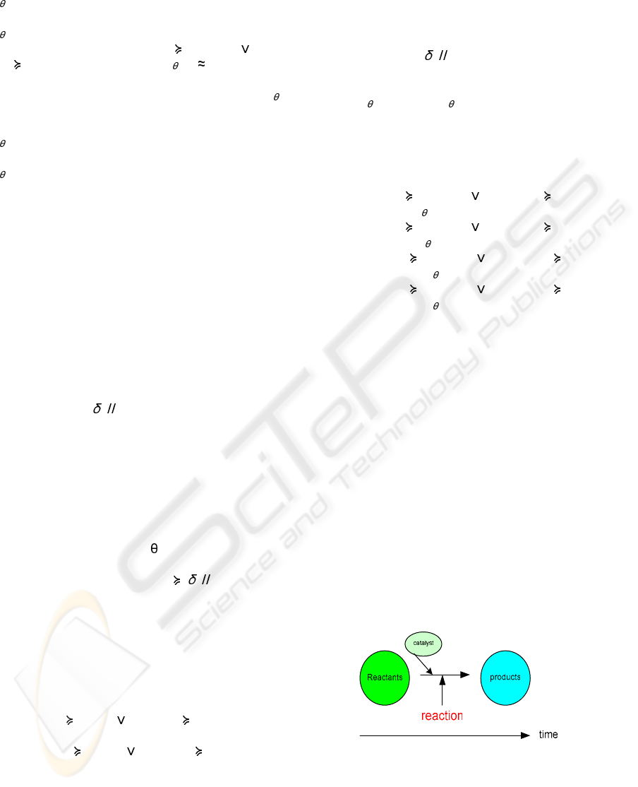
We deal with the rate of the data change, and we
see the fact about the catalyst in the chemical
reaction, that is, the catalyst can activate the rate of
the chemical reaction to make it happen faster. So
we look at the character of the catalyst in the
chemical reaction in (Liska and Pryde 1984;
Harrison, Mora et al. 1991; Freemantle 1995;
Robinson, Odom et al. 1997; Snyder 1998). Not all
of the chemical reaction has the catalyst. We think
that some events act as the catalyst. The amount of
the catalyst at the time before the reaction time is
higher than its amount at the reaction time and its
amount at the time after the reaction time is higher
than its amount at the reaction time. So we compare
the amount of the event of the attribute of
consideration at the previous time point with its own
amount at the current time point. And we also
compare the amount of the event of the attribute of
consideration at the post time point with its own
amount at the current time point.
Figure 2: The chemical reaction include the catalyst
We look at the time that the reaction time as the
reference event. We see that the amount of the
reactants at the previous time point is higher than the
amount of the reactants at the current time point.
MINING THE RELATIONSHIPS IN THE FORM OF PREDISPOSING FACTOR AND CO-INCIDENT FACTOR IN
TIME SERIES DATA SET BY USING THE COMBINATION OF SOME EXISTING IDEAS WITH A NEW IDEA
FROM THE FACT IN THE CHEMICAL REACTION
533

And also the amount of the catalyst at the previous
time point is higher than the amount of the catalyst
at the current time point. The amount of the products
at the post time point is higher than the amount of
the products at the current time point. We look at the
reactant and the catalyst at the previous time point as
the predisposing factor and look at the product as the
co-incident factor. The fact about the catalyst is it
will not be transformed to be the product, so after
the reaction finish, we will get the catalyst back. We
will see the amount of the catalyst at the post time
point is higher than the amount of the catalyst at the
current time point. So we look at the catalyst at the
post time point as the co-incident factor as well.
4 EXPERIMENTS
We apply our method with one OSS data set which
consists of 17 attributes (Project name, Month-Year,
Rank0, Rank1, Page-views, Download, Bugs0,
Bugs1, Support0, Support1, Patches0, Patches1,
Tracker0, Tracker1, Tasks0, Tasks1, CVS. This data
set consists of 41,540 projects, 1,097,341 records
4.1 Results
We set the rate of the data change threshold of the
Download attribute and the rest of all of the other
attributes as 1.5.
4.1.1 In case without considering the slope
rate direction of the Download
attribute
Predisposing Factor(s): Tasks0, Tasks1, CVS
Co-incident Factor(s): Support0, Support1,
Patches0, Patches1
4.1.2 In case considering the slope rate
direction of the Download attribute
The acceleration of the Download attribute
Predisposing Factor(s): none
Co-incident Factor(s): Bugs0, Bugs1, Support0,
Support1, Patches0, Patches1, Tracker0, Tracker1
The deceleration of the Download attribute
Predisposing Factor(s): Bugs0, Bugs1, Support0,
Support1, Patches0, Tracker0, Tasks0, Tasks1, CVS
Co-incident Factor(s): Support1
5 CONCLUSION
The combination of the existing methods and the
new idea from the fact seen in the chemical reaction
to be our new algorithms can be used to mine the
predisposing factor and co-incident factor of the
reference event of interest very well. As seen in our
experiments, our propose algorithms can be applied
with both the synthetic data set and the real life data
set. The performance of our algorithms is also good.
They consume execution time just in linear time
scale and also tolerate to the noise data.
REFERENCES
Freemantle, M., 1995. Chemistry in Action. Great Britain,
MACMILLAN PRESS.
Harrison, R. M., Mora S., et al., 1991. Introductory
chemistry for the environmental sciences. Cambridge,
Cambridge University Press.
Last, M., Klein Y., et al., 2001. Knowledge Discovery in
Time Series Databases. In IEEE Transactions on
Systems, Man, and Cybernetics 31(1): 160-169.
Liska, K. and Pryde L., 1984. Introductory Chemistry for
Health Professionals. USA, Macmillan Publishing
Company.
Robinson, W. R., Odom J., et al., 1997. Essentials of
General Chemistry. USA, Houghton Mifflin
Company.
Roddick, J. F. and Spiliopoulou M., 2002. A Survey of
Temporal Knowledge Discovery Paradigms and
Methods. In IEEE Transactions on Knowledge and
Data Mining 14(4): 750-767.
Snyder, C. H. 1998. The Extraordinary Chemistry of
Ordinary Things. USA, John Wiley & Sons, Inc.
ICEIS 2004 - ARTIFICIAL INTELLIGENCE AND DECISION SUPPORT SYSTEMS
534