A QUALITATIVE MODEL OF THE INDEBTEDNESS FOR THE
SPANISH AUTONOMOUS REGIONS
Luis Jimenez, Juan Moreno-Garcia, Jose Jesus Castro-Schez, Victor R. Lopez, Jose Ba
˜
nos
Universidad de Castilla-La Mancha
Departamento de Informatica, Departamento de Economia y Empresa
E.S.I. de Ciudad Real, E.U.I.T.I. de Toledo, F.CC.E. y E. de Albacete
Keywords:
approximate reasoning, linguistic models, economy models, fuzzy logic.
Abstract:
This work shows a fuzzy model of the indebtedness for the Spanish autonomous regions that is obtained using
approximate reasoning and induction methods. So, the algorithm ADRI (M. Delgado, 2001; Jimenez, 1997)
is used to induce a linguistic model composed by a set of fuzzy rules. The quality of this linguistic model will
be checked and its interpretation will be shown.
1 INTRODUCTION
Currently, the technology offers the possibility to
work efficiently with a lot of data. We can to use in-
duction methods to detect the relations between sev-
eral variables without previous hypothesis.
In this work we make use of an induction method
to study the indebtedness for the Spanish autonomous
regions from 1986 to 2000. Our aim will be to find
the temporal relations among the indebtedness of a
region in a year t and the non financial revenues and
the type of interest of that year and the indebtedness
of the region in the year t − 1. To do this, we have
a set of data owning to J. Ba
˜
nos, P. Cillero and V.R.
L
´
opez (J. Ba
˜
nos, 2001) that was obtained from several
reliable source, Spanisn National Bank, Ministry of
Finance and Statistic National Institute and Statistic
National Institute (INE).
Our intention is to obtain a model that, in one hand,
will be understandable without difficulty, and in the
other hand, can be directly developed from empir-
ical observation. Thus, we are interested in tech-
niques that obtain models given by using fuzzy rules
with linguistic variables (Zadeh, 1975; M. Sugeno,
1991). We suggested make use of the induction algo-
rithm ADRI (M. Delgado, 2001) in order to obtain the
model that describes the run of the Spanish regions in-
debtedness. This algorithm obtains a set of linguistic
rules from data.
The next section gives a background knowledge of
the induction algorithm ADRI. In section 3 the model
of the indebtedness for the Spanish autonomous re-
gions is obtained. After that, an interpretation of this
model is exposed in Section 4. Finally, the conclu-
sions are shown.
2 ADRI: AN INDUCTION
METHOD
ADRI is a generalization of the regression technique.
Firstly, we show some definitions used in this paper
and, after, we describe briefly the ADRI induction
method.
Let S = {s
1
, s
2
. . . s
n
} be a set of data defined for
the set of values that takes a set of variables X =
{X
1
, X
2
. . . X
d
}, thus, s
i
= {x
1
i
, x
2
i
. . . x
d
i
, y
i
}.
Let F be a function that only is known in the set
S, such that, F (s
i
) = y
i
. The aim of the regres-
sion methods, expressed by means of a parameterized
function F
0
, is to minimize the distance between the
real output value y
i
= F (s
i
) and its estimated value
using F
0
(s
i
).
The regression methods are different to the classi-
fication methods. The regression methods consider
continuous output values instead of a set of cate-
gories in the classification methods. From this point
of view, the classification methods could be consid-
ered a particularization of the regression methods.
Methods based on the successive partitioning of the
problem domain (for example, the decision trees ID3
(Quilan, 1986)) are used like technique of regression
for restrictions in Classification and regression trees
275
Jimenez L., Moreno-Garcia J., Jesus Castro-Schez J., R. Lopez V. and Baños J. (2004).
A QUALITATIVE MODEL OF THE INDEBTEDNESS FOR THE SPANISH AUTONOMOUS REGIONS.
In Proceedings of the Sixth International Conference on Enterprise Information Systems, pages 275-280
DOI: 10.5220/0002616502750280
Copyright
c
 SciTePress

(CART) (J. Breiman, 1984).
CART is based on a sequence of questions and its
possible answers (structured in tree form) over the
variable values that define the problem. CART ob-
tains a separate divisions SR = {r
1
, r
2
. . . r
p
} of the
domain of each variable of the problem. It splits the
domains by means of the answers to the questions that
carries out. The algorithm used in this work gener-
alizes the divisions obtained in CART by means of
fuzzy logic (Zadeh, 1965).
In this work, we build the Classification and Re-
gression Fuzzy Tree for the Spanish regions indebt-
edness problem and obtain the searched model given
by means of a set of fuzzy rules. It will be the param-
eterized function F
0
obtained by ADRI.
Now, we expose how the set of rules is obtained.
Let A
T
be a fuzzy set of the tree node T defined over
the set of data S. The root node contains all data of
the set S, and its membership function is A
T
: S → 1.
The output associated to the node T is defined using
the membership grade A
T
(s
i
) of each data s
i
and the
output y
i
(equation 1).
F
00
(T ) =
P
n
i=1
A
T
(s
i
)
m
∗ y
i
P
n
i=1
A
T
(s
i
)
m
(1)
where A
T
(x) is calculated as min
d
j=1
A
j
T
(x
j
)
and A
j
T
(x
j
) is the membership function of a
fuzzy set defined over the domain of the j-th vari-
able.
Equation 2 calculates the estimated error E(T ) of
a node T .
E(T ) =
P
n
i=1
(F
00
(T ) − y)
2
∗ A
T
(s
i
)
m
P
n
i=1
A
T
(s
i
)
m
(2)
Now, our problem is how to establish a set of ques-
tions to divide the node T . These questions are car-
ried out for each variable, thus, a binary division of
the node T is obtained for each one of the variables.
We suppose binary division for the fuzzy set associ-
ated to the node T (by means of the fuzzy set A
j
T
of
the variable j), that is, p
j
T
= {B(x), C(x)} where
A
j
T
= B(x) + C(x). This partition creates two
new nodes and two new fuzzy sets associated to them
(Equations 3 and 4).
A
T
1
(s
i
) = min(A
T
(s
i
), B(x
j
i
)) (3)
A
T
2
(s
i
) = min(A
T
(s
i
), C(x
j
i
)) (4)
Thus, the obtained rules with this fuzzy sets are:
IF variable
j
IS A
T
1
THEN .....
ELSE
IF variable
j
IS A
T
2
THEN ..
Following the ADRI algorithm, we obtain the pro-
portion of the fuzzy sets B(x) and C(x) in relation to
the fuzzy set A
j
T
(Equations 5 and 6).
P (T
1
) =
P
n
i=1
B(x
j
i
)
P
n
i=1
A
j
T
(x
j
i
)
(5)
P (T
2
) =
P
n
i=1
C(x
j
i
)
P
n
i=1
A
j
T
(x
j
i
)
(6)
The quality of this partition is estimated with the
equation 7.
C(T, p
j
) = (E(T
1
)P (T
1
)) + (E(T
2
)P (T
2
)) (7)
where p
j
is the fuzzy partition of the j-th vari-
able.
The selected partition is the one that has the mini-
mum value C(T, p
j
). This technique generates a hier-
archical fuzzy partition in each one of the variables to
obtain the questions. This process of division obtains
the relevant variables to define the model. The mech-
anism of division is stopped when some condition is
verified. In our case, the condition is that the error is
less than a constant c (equation 8).
ERROR = max
T ∈
T
{E(T )} 6 c (8)
where
T is the set of tree leaves, thus, each
leaves is a fuzzy region of the model.
Equation 9 calculates the final output value for each
input value s
i
.
F
00
(s) =
P
t∈T
A
T
(s)
m
∗ F
00
(T )
P
t∈T
A
T
(s)
m
(9)
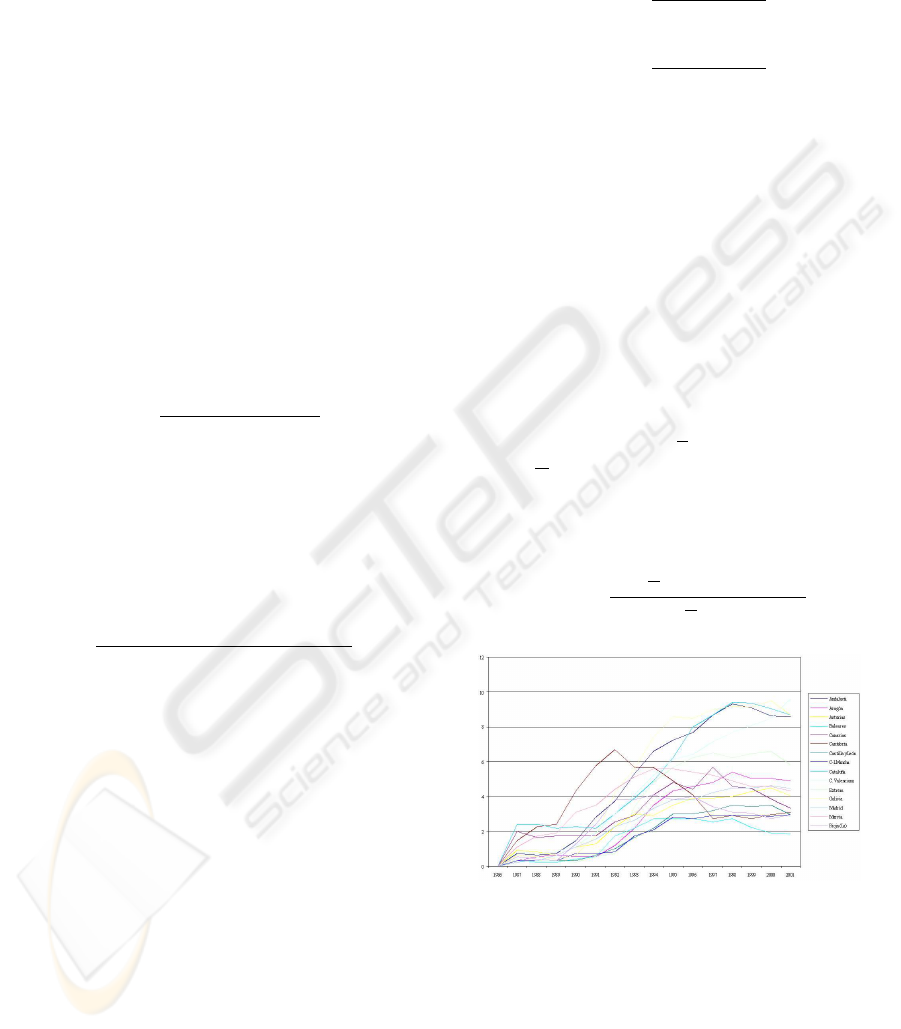
Figure 1: Indebtedness for Spanish autonomous regions
from 1986 to 2000
The interested reader is referred to M. Delgado
(M. Delgado, 2001).
3 INDEBTEDNESS MODEL
We want to obtain a model that shows the indebt-
edness for the Spanish autonomous regions from
ICEIS 2004 - ARTIFICIAL INTELLIGENCE AND DECISION SUPPORT SYSTEMS
276

1986 to 2000 (Figure 1). The output variable (the
modelled variable) is the indebtedness for the Span-
ish autonomous region in the year t, and the input
variables are the region indebtedness of the previ-
ous year D/P IB(t − 1), the non financial revenues
IN F/P IB(t) and the type of interest T (t). Thus,
the searched function F is shown in Equation 10.
F (D/P IB(t − 1), INF/P IB(t), T (t)) (10)
The fuzzy model F
0
is developed using the Clas-
sification and Regression fuzzy tree (ADRI). A fuzzy
rule consist of two components, the first one is the an-
tecedent and the second one is the consequent. These
components show the cause-effect relation. The an-
tecedent is formed for aggregation of fuzzy proposi-
tions, such as X is A, where X is the input variable
and A is the fuzzy set defined over its domain. In this
work, the membership function of the fuzzy sets are
trapezoidal functions (see Equation 11). This mem-
bership function is adequate for our problem due to it
is one of the most simple membership function, and
it is easy to construct from the fuzzy sets obtains by
using ADRI (ADRI is defined over trapezoidal sets).
The change to other membership function not implies
substantial modifications.
A(x, a, b, c, d) =













0 x 6 a
x−a
b−a
a < x < b
1 b 6 x 6 c
d−x
d−c
c < x < d
0 x > d
(11)
Our aim is to define a system of linguistic rules,
since linguistic labels must be associated to each one
of the fuzzy sets in which is divided the domain of
each input variable (Tables 1, 2 and 3). Each row of
these tables define a linguistic value. The numbers
which appear in the first column of the tables are the
four values that define the trapezoidal function of the
linguistic value given in its associated second column.
Thereby, we get a set of linguistic variables (Zadeh,
1975).
Table 1: Linguistic Variable D/PIB
[8.00, 8.48, MAX, MAX] Extremely Big
[6.45, 7.20, 8.00, 8.48] Very Big
[3.53, 4.50, 6.45, 7.20] Big
[1.50, 2.10, 3.53, 4.50] Norm
[0.80, 1.10, 1.50, 2.10] Small
[0.40, 0.60, 0.80, 1.10] Very Small
[MIN, MIN, 0.40, 0.60] Extremely Small
The model acquired by ADRI may be observed in
Table 4. Each row is a rule with EB is Extremely Big,
V B is Very Big, B is Big, N is Norm, S is Small,
Table 2: Linguistic Variable INF/PIB
[14.08, 15.62, MAX, MAX] Big
[8.68, 10.84, MAX, MAX] Norm or Big
[8.96, 10.84, 14.02, 15.62] Norm
[MIN, MIN, 8.68, 10.84] Small
Table 3: Linguistic Variable T
[11.05, 12, 49, MAX, MAX] Big
[8.22, 9.65, 11.05, 12.49] Norm
[MIN, MIN, 5.87, 9.65] Small
V S is Very Small and ES is Extremely Small. These
rules are arranged in a decreasing way according to
the percentage of data that are correctly classified by
the rule. The first number indicates the index of the
rule, the following four are the values that the input
variable take, the sixth the rule error and the last per-
centage of instances that has been correctly classified.
Thus, the rule 10 covers the 7.4% of the data, it has a
error of 0.04%, and it could be read as:
IF D/P IB(t − 1) is Big AND IN F/P IB(t)
is Small AND T (t) is Small THEN
D/P IB(t) is 4.55
Now, let us look at how the model responds to a
situation. Table 5 shows how is carried out the infer-
ence from the data about Andalusia in 1993. Each
row of this table is a rule of the model (see Ta-
ble 4). The first number indicates the index of the
rule, the following three are the values that the in-
put variables (D/P IB(t − 1), INF/P (t) and T (t))
take in each rule (value 1), the fifth the minimum
membership grade for the input variables and the last
the value of the output variable. The real output is
D/P IB(t) = 6.6. The data about Andalusia, input
of the model, are 5.3, 18.96 and 10.17 for the input
variables D/P IB(t − 1), INF/P IB and T (t) re-
spectively. The output value obtained by the model is
D/P IB(t) = 6.23.
The cell (1, D/P IB(t − 1)) contains the mem-
bership grade of the value 5.3 to the fuzzy set
[0.80, 1.10, 1.50, 2.00] labelled as Small. The value
into the cell (9, min) represents the minimum value
of the membership of the input values set to the rule
9 (row 9). The cell value (9, D/P (T )) is the output
of the rule 9 multiplied by the cell value (9, min).
The output value is the weighted average of all out-
puts times the min column.
In Figures 2 to 16 we show the predictive perfor-
mance of the model. Each Figure presents the results
of a Spanish region, the real and obtained indebted-
ness (Y
axis) in each year (X axis). The real in-
debtedness is represented by a continuous line. The
A QUALITATIVE MODEL OF THE INDEBTEDNESS FOR THE SPANISH AUTONOMOUS REGIONS
277

Table 4: Obtained Model
N D(t-1) I(t) T(t) D(t) E C
13 ES 0.51 0.03 11.4
5 N N 3.43 0.09 10.7
12 VS 1.06 0.06 10.2
1 S 2.23 0.10 9.4
3 N S S 3.20 0.07 9.3
4 N B 3.18 0.09 8.8
10 B S S 4.55 0.04 7.4
7 EB 8.97 0.02 6.8
11 B N or B S 5.43 0.09 5.4
8 B S N 4.94 0.06 5.3
9 B N or B N 6.23 0.06 4.2
6 VB 7.76 0.05 4.0
14 N N or B S 3.28 0.06 3.7
2 B B 4.96 0.07 2.3
15 N B S 5.10 0.05 0.8
discontinuous line is the obtained indebtedness using
the presented method.
The Spanish regions indebtedness in the year 2001
have been inferred making use of the model (see Ta-
ble 5) and composed with the real values. In Table
6 we show the result obtained, where each row is a
Spanish region (A.R.),D(t − 1), I(t) and T (t) are the
input variables D/P IB(t − 1), INF/P (t) and T (t)
respectively, and Ob. D(t) and R. D(t) are the ob-
tained and real output variable D/P IB(t).
4 INTERPRETATION OF THE
MODEL
The obtained model allows to make an analysis of
the indebtedness for the Spanish autonomous regions
from 1986 to 2000. The aim of our analysis is double:
in one hand, find the rules that define the most of the
study cases; and in the other hand, get the influence
of each one of the input variables in the indebtedness
prediction problem.
We can observe that the rules 13, 12, 1, 7 and 6
classify correctly the 11.4%, 10.23%, 9.38%, 6.78%
and 3.98% of the whole set of cases respectively, i.e.,
41,77%. On the other hand, we can also observe that
the output of the model (D/P IB(t)) in this rules only
depend on the value of the input variable D/P IB(t−
1). Thus, the behavior of the D/P IB value in time t
is very dependent of the value in time t − 1. It causes
an inertial behavior to the model, that is, when the
variable input D/P IB(t − 1) has small, medium or
big values the output value is small, medium or big.
The rules 5, 4 and 2 (whose antecedent depend
Table 5: Inference process for Andalusia
R D/P(t-1) INF/P(t) T(t) min D/P(T)
1 0 1 1 0 0
2 1 1 0 0 0
3 0 0 0 0 0
4 0 1 0 0 0
5 0 1 1 0 0
6 0 1 1 0 0
7 0 1 1 0 0
8 1 0 1 0 0
9 1 1 1 1 6.23
10 1 0 0 0 0
11 1 1 0 0 0
12 0 1 1 0 0
13 0 1 1 0 0
14 0 0 0 0 0
15 0 1 0 0 0
on the variables D/P IB(t − 1) and T (t)) clas-
sify correctly the 10.74%, 8.83% and 2.30% of the
whole set of cases, i.e., 21,87%. This means that
the D/P IB(t) value is corrected by the T (t) values
when the D/P IB(t) values are Norm or Big.
Finally, the INF/P IB(t) variable is used in the
36.36% of the data.
Thus, we deduce that the indebtedness for the
Spanish autonomous regions in a year t depend on
basically of the indebtedness for the Spanish au-
tonomous regions in a year t − 1, lightly corrected for
the type of interest and minorly for the non financial
revenues.
5 CONCLUSION
This work presents a methodology to define mod-
els. This methodology don’t need knowledge a priori,
except in the variable definition. This methodology
uses induction technique to obtain the models that are
qualitative and are based on fuzzy logic.
To validate the methodology we obtain a linguis-
tic model of the indebtedness for the Spanish au-
tonomous regions. A brief analysis is doing to show
the behavior of the model. Of the obtained result we
conclude that the methodology obtains a good first ap-
proximation to the searched model. The understand-
ing of the model is possible because the model is qual-
itative (linguistic labels).
ICEIS 2004 - ARTIFICIAL INTELLIGENCE AND DECISION SUPPORT SYSTEMS
278

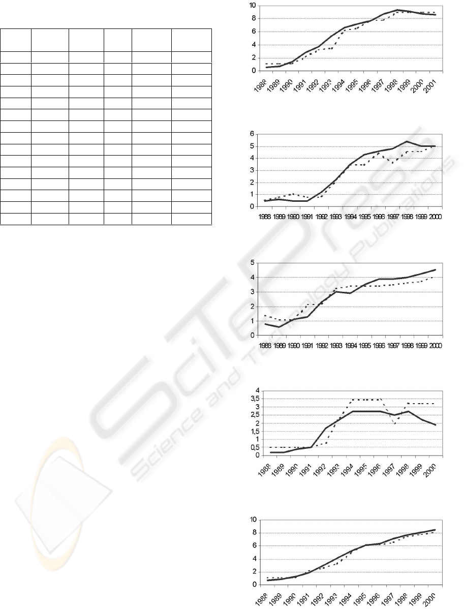
Table 6: Indebtedness values obtained by the model for each
Spanish region in the year 2001
Ob. R.
A.R. D(t-1) I(t) T(t) D(t) D(t)
An. 8.58 20.44 4.5 8.9668 8.8213
Ar. 4.88 10.23 4.5 5.1806 4.8286
As. 4.05 7.10 4.5 3.9534 3.9212
B. 1.85 5.93 4.5 2.8687 1,6450
Cn. 3.30 16.47 4.5 5.1041 3.3405
Ct. 3.08 10.24 4.5 3.2585 2.9857
CL. 2.95 13.12 4.5 3.2837 2.9152
CM. 2.93 12.71 4.5 3.2837 2.8815
Cat. 8.70 11.11 4.5 8.9668 8.7626
CV. 9.58 12.69 4.5 8.9668 9.6902
E. 5.83 15.17 4.5 5.426 5.9000
G. 8.68 19.11 4.5 8.9668 8.8971
M. 4.48 6.36 4.5 4.4296 4.2426
Mu. 4.30 10.38 4.5 4.758 4.3415
R. 2.93 8.91 4.5 3.1953 2.8055
ACKNOWLEDGEMENTS
This work has been funded by the Spanish Ministry of
Science and Technology and Junta de Comunidades
de Castilla-La Mancha under Research Projects ”DI-
MOCLUST” TIC2003-08807-C02-02 and PREDA-
COM PBC-03-004.
REFERENCES
J. Ba
˜
nos, P. Cillero, V. L. (2001). Un modelo de endeu-
damiento economico. Presupuesto y gasto publico, n
o
26, 2001, 161-172.
J. Breiman, J. Friedman, R. O. S. (1984). Classification and
regression tree. Monterey, Ca:Wadsworth.
Jimenez, L. (1997). Modelizacion difusa de sistemas me-
diante tecnicas inductivas. Tesis Doctoral, ETSI Uni-
versidad de Granada.
M. Delgado, A.F. Skarmeta, L. J. (2001). A regression
methodology to induce a fuzzy Model. International
Journal of Intelligent Systems Vol 16, n
o
2, 169-190,
February.
M. Sugeno, T. Y. (1991). A fuzzy-logic based approach to
qualitative modelling. IEEE Trans Sys Man Cyber,
vol 1, 7-31.
Quilan, J. (1986). Induction of decision tree. Machine
Learning, vol 1, 81-106.
Zadeh, L. (1965). Fuzzy sets. Inform Control, 338-353.
Zadeh, L. (1975). The concept of linguistic variable and its
applications to approximate reasoning part I,II and
III. Inform Sci vol 8 and 9, 199-249 301-357 43-80.
Figure 2: Andalusia Indebtedness (An.)
Figure 3: Aragon indebtedness (Ar.)
Figure 4: Asturias Indebtedness (As.)
Figure 5: Balearic Islands Indebtedness (B.)
Figure 6: Valencian Community Indebtedness (C.V.)
A QUALITATIVE MODEL OF THE INDEBTEDNESS FOR THE SPANISH AUTONOMOUS REGIONS
279

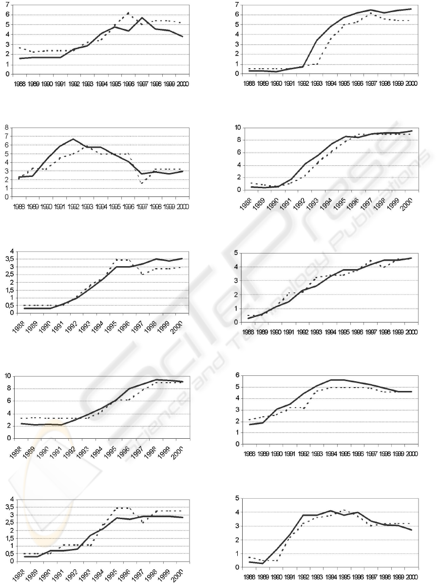
Figure 7: Canary Isles Indebtedness (Cn.)
Figure 8: Cantabria Indebtedness (Ct.)
Figure 9: Castile and Leon Indebtedness (CL.)
Figure 10: Catalonia Indebtedness (Cat.)
Figure 11: Castile and La Mancha Indebtedness (CM.)
Figure 12: Extremadura Indebtedness (E.)
Figure 13: Galicia Indebtedness (G.)
Figure 14: Madrid Indebtedness (M.)
Figure 15: Murcia Indebtedness (Mu.)
Figure 16: La Rioja Indebtedness (R.)
ICEIS 2004 - ARTIFICIAL INTELLIGENCE AND DECISION SUPPORT SYSTEMS
280