OPTIMIZATION OF NEURAL NETWORK’S TRAINING SETS
VIA CLUSTERING: APPLICATION IN SOLAR COLLECTOR
REPRESENTATION
Luis E. Zárate*, Elizabeth Marques Duarte Pereira**,
Daniel Alencar Soares*, João Paulo D. Silva*, Renato Vimieiro*,
Antonia Sonia Cardoso Diniz***
*Applied Computational Intelligence Laboratory (LICAP)
**Energy Researches Group (GREEN)
***Energy Company of Minas Gerais (CEMIG)
Pontifical Catholic University of Minas Gerais (PUC)
Av. Dom José Gaspar, 500, Coração Eucarístico
Belo Horizonte, MG, Brasil, 30535-610
Keywords: Artificial Intelligence, Artificial Neural Networks, Solar Energy, Clustering, Thermosiphon.
Abstract: Due to the necessity of new ways of energy producing, solar collector systems have been widely used
around the world. There are mathematical models that calculate the efficiency of those systems; however
these models involve several parameters that may lead to nonlinear equations of the process. Artificial
Neural Networks have been proposed in this work as an alternative of those models. However, a better
modeling of the process by means of ANN depends on a representative training set; thus, in order to better
define the training set, the clustering technique called k-means has been used in this work.
1 INTRODUCTION
In a reality where natural resources are becoming
scarce, associated with the population increasing, the
traditional ways of energy producing (hydroelectric
power plants) may not be sufficient. Therefore some
alternative ways of energy producing are proposed;
and among them, there are solar energy systems.
Solar energy systems, specifically water heaters,
have considerable importance in the substitution of
traditional electrical systems. The most widely used
solar energy systems are known as thermosiphon
systems; which are cost competitive with those
conventional energy systems available everywhere.
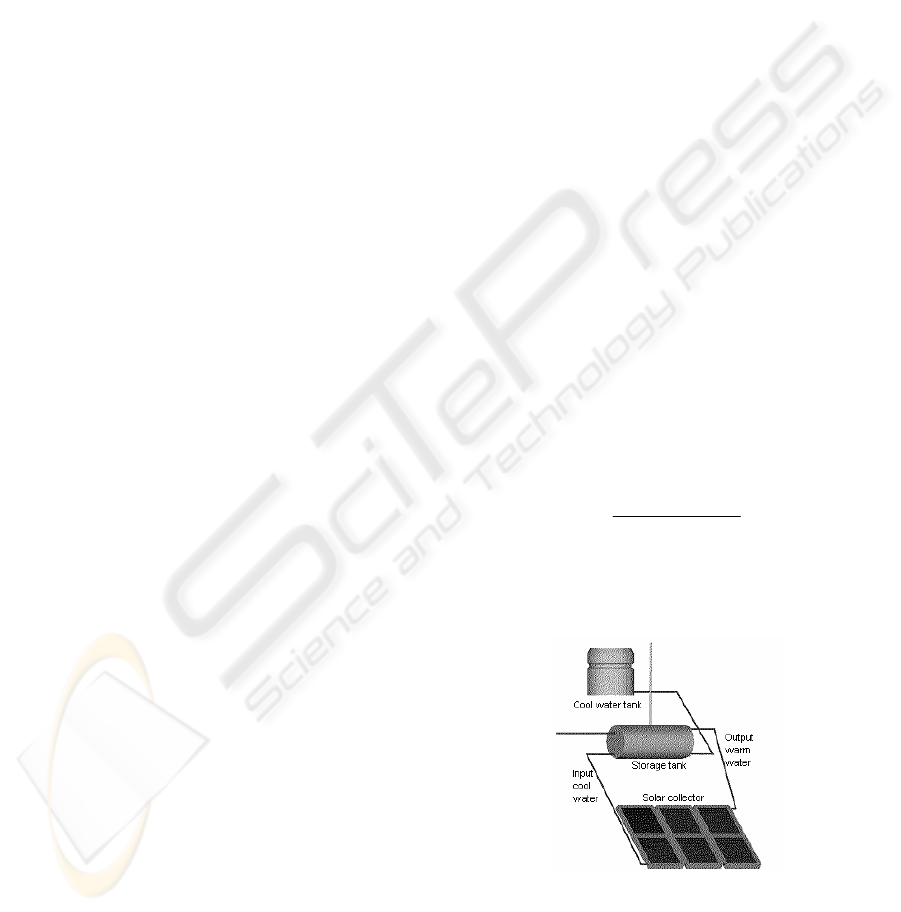
In Figure 1, a schematic diagram of thermosiphon
system is represented; its main component is the
collector plate. Numerous researchers
(Morrison &
Ranatunga 1980; Huang 1984; Kudish, Santaura &
Beaufort 1985
) investigate the performance those
systems, both experimentally and analytically. The
efficiency of thermosiphon systems can be obtained
by means of the equation
extern
inoutp
GA
TTcm )( −
=
&
η
(1)
where η is efficiency, m, the flow rate, c
p
, the heat
capacity of water, T
out
, the output water temperature,
T
in
, the input water temperature, G, solar irradiance
and A
extern
is the area of the collector.
Figure 1: Schematic diagram of thermosiphon system.
The solar collector efficiency depends on some
structural aspects like its position, the material of its
components and thermal insulation. Efficiency is
obtained by means of experiments that use some
process parameters like output water temperature,
147
E. Zárate L., Marques Duarte Pereira E., Alencar Soares D., Paulo D. Silva J., Vimieiro R. and Sonia Cardoso Diniz A. (2004).
OPTIMIZATION OF NEURAL NETWORK’S TRAINING SETS VIA CLUSTERING: APPLICATION IN SOLAR COLLECTOR REPRESENTATION.
In Proceedings of the Sixth International Conference on Enterprise Information Systems, pages 147-152
DOI: 10.5220/0002606001470152
Copyright
c
 SciTePress

ambient temperature, input water temperature, solar
irradiance and flow rate. Thus, for new operational
conditions, new experiments must be made in order
to recalculate the efficiency. There are mathematical
models that avoid those experiments (Kudish,
Santaura & Beaufort 1985), but they have the
discouraging aspect of involving several parameters
that may lead to non-linearity.
Linear regression has been proposed as alternative to
those complex mathematical models. However that
technique may introduce estimative errors in actual
and future values due to its limitation in better
working with linearly correlated values.
In the last years, Artificial Neural Networks (ANN)
have been proposed as powerful computational tools
due to their facility in solving non-linear problems,
generalizing what they have learnt, besides the low
time of processing that can be reached when the nets
are in operation. Some researches discuss the use of
ANN to represent termosiphon systems (Kalogirou
2000; Kalogirou, Panteliou & Dentsoras 1999;
Zárate et al. 2003a; Zárate et al. 2003b). In Zárate et
al. 2003a, a net trained with 603 data has been
presented, however the time spent to train this net is
not satisfactory. In Zárate et al. 2003b, statistical
analysis is adopted with the objective of building a
reduced but better defined training set. In Moreira
and Roisenberg 2003, an alternative solution, based
in genetic algorithm, is presented as an alternative of
reducing the training set; but the needed time to
obtain the optimal training set makes this technique
not satisfactory.
The usage of ANN to model solar collectors has
several advantages over other techniques, like not
needing linearly correlated data and their capacity of
generalization in order to deal of new data values.
ANN are presented here, besides the clustering
technique known as k-means, used to reduce and
better define the training set.
This paper is organized in six sections. In the second
one, solar collectors are physically described. In the
third section, the process of collecting data from the
solar collector is presented. In the fourth one,
clustering technique is presented. In the fifth section,
modeling by means of ANN is discussed. And
finally, conclusions are presented.
2 PHYSICAL DESCRIPTION OF
THE SOLAR COLLECTOR
The working principles of thermosiphon systems are
based on thermodynamic laws (Duffie & Beckman
1999). In those systems water circulates through the
solar collector due to the natural density difference
between cooler water in the storage tank and warmer
water in the collector. Although they demand larger
cares in their installation, thermosiphon systems are
of extreme reliability and lower maintenance. Their
application is restricted to residential installations
and to small commercial and industrial installations.
Thermosiphon system structure is presented in
Figure 1.
Solar irradiance reaches the collectors, which heat
up water inside them, decreasing the density of
heated up water. Thus cooler and denser water
forces warm water to the storage tank. Since this is a
constant process, the water flow happens between
the storage tank and the collector, resulting in a
natural circulation called “thermosiphon effect”.
3 COLLECTING DATA FROM
THE SOLAR COLLECTOR
Collected data refer to a typical solar collector and
have been obtained by means of experiments in
different ambient situations, under ASHRAE
standards (ASHRAE 93-86 RA 91). During three
days of a characteristic period of the year for those
experiments, measurements have been realized
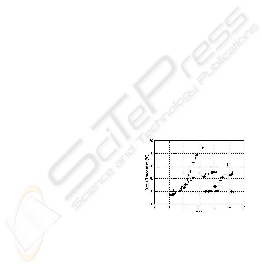
several times per day. Figure 2 shows a graphic
where the relation between output temperature of
water (T
out
) and the hours during the day (hours) can
be observed. Notice that the collected data are
representative for different operating points and
output temperatures.
Figure 2: Collected output water temperatures.
In order to verify the non-linearity of the collected
data, some graphics have been built, like the one
presented in Figure 3, however linearity in those
data has been noticed. Despite that linearity, ANN
are presented here as an alternative to model solar
collectors with more precision than other techniques
like linear regression.
ICEIS 2004 - ARTIFICIAL INTELLIGENCE AND DECISION SUPPORT SYSTEMS
148

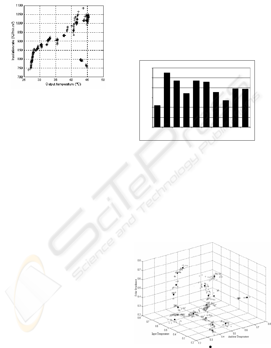
Figure 3: Solar irradiance X output water temperature.
The total number of collected data equal 631; those
data include values of solar irradiance (G), ambient
(T
amb
), input (T
in
) and output (T
out
) temperatures.
Table I.1 (in the append) shows a sample composed
by 15 of those collected data. A subset composed by
30 data has been extracted from the original set in
order to be used as validation set which is used later.
Thus the new training set contains 601 data.
A reduced and better-defined training set must
continue representing the problem, maintaining the
capacity of generalization of the net, tolerable errors
and permitting the reduction of time spent in the
training process. In Zárate et al. 2003b, statistical
analysis has been used to reduce the training set,
resulting in 84 data. The clustering technique called
k-means has been used in this work to reduce the
training set, maintaining its capacity of represent the
problem.
4 CLUSTERING WITH K-MEANS
The k-means algorithm is one of the several
techniques of clustering. It divides n data into k
clusters, where k is a constant not defined by the
algorithm. The result of this algorithm is a frame
where all the objects present in a cluster have
considerable similarity among them and a great
dissimilarity to objects present in other clusters.
Each cluster has a center point, which has the
principal characteristics of the group. In the center
point, the sum of distances of all objects in that
cluster is minimized.
4.1 Selecting data for the training
In order to build a representative training set, the k-
means algorithm, described above, has been used in
the set composed by 601 data. The technique has
been applied identifying clusters in which data have
similar characteristics. As the number k of clusters
must be explicitly given to the algorithm, k value has
been varied from 10 to 100. For each test with a
different number of clusters, the distance between
each point in data set to each cluster center point has
been calculated. Figure 4 shows average distances
between all points of each cluster and the center
points of neighbor clusters, for all the tested
quantities of clusters.
0,6
0,62
0,64
0,66
0,68
0,7
0,72
10 20 30 40 50 60 70 80 90 100
Figure 4: Average distances between the points of
each cluster and the neighbor clusters.
Higher average distances between the points of each
cluster and the center points of neighbor clusters
characterize better-defined clusters. Considering
this, the set divided in 20 clusters has been chosen.
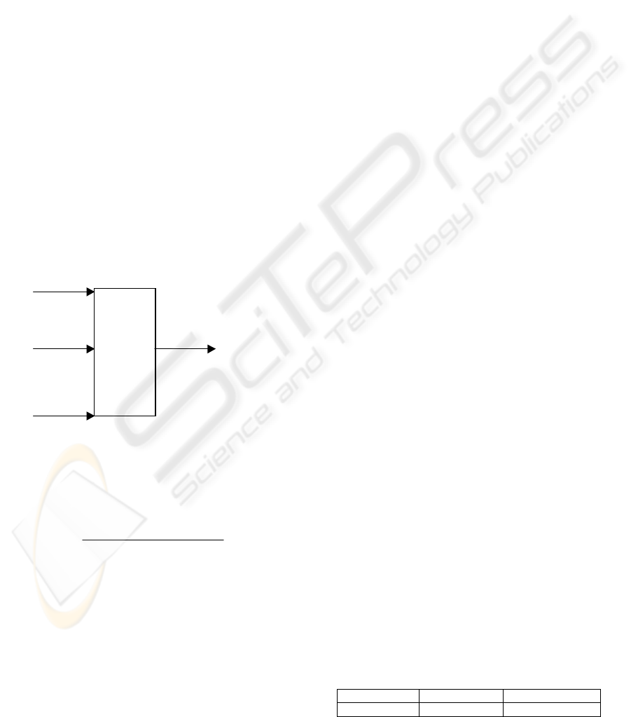
After determining the optimal number k of clusters,
a technique to select data present in the clusters has
been applied. Although most representative
characteristics are present in the center point of each
cluster, this center point may not correspond to a
real point in the data set. Thus, for each cluster, the
point closest to the center point has been chosen
resulting in 20 sets. Figure 5 shows, graphically, the
data set divided in 20 clusters.
Figure 5: Clusters centers points ( ) and data values (+).
OPTIMIZATION OF NEURAL NETWORK’S TRAINING SETS VIA CLUSTERING: APPLICATION IN SOLAR
COLLECTOR REPRESENTATION
149

5 NEURAL REPRESENTATION
OF SOLAR COLLECTOR
Multi-layer ANN have been used in this work. The
values of entries are presented to the hidden layer
and satisfactory answers are expected to be obtained
from the output layer. The most suitable number of
neurons in the hidden layer is still a non-solved
problem, although researches discuss some
approaches. In Kovács 1996, the suggested number
of hidden neurons is 2n+1, where n is the number of
entries. In the other hand, the number of output
neurons equals the number of expected answers
from the net.
Input water temperature (T
in
), solar irradiance (G)
and ambient temperature (T
amb
) are variables used as
entries to the ANN. The output water temperature
(T
out
) is the wanted output from the net. In this work,
ANN represent the thermosiphon system according
to the following formula
out
ANN
ambin
TGTTf ⎯⎯→⎯),,( (2)
The structure of the ANN in this work is
schematically represented as shown in the Figure 6.
The net contains seven hidden neurons (i.e. 2n+1)
and one neuron in the output layer, from which the
output water temperature is obtained.
T
amb
T
in
G
T
out
ANN
Figure 6: Schematic diagram of ANN.
Supervised learning has been adopted to train the
net, specifically, the widely used algorithm known
as backpropagation. Nonlinear sigmoid function has
been chosen, in this work, as the axon transfer
function
∑
−
+1
1
=
x Weigths
exp
Entries
f
(3)
5.1 Preparing data for training
The largest effort to get a trained net generally lies
on collecting and pre-processing the input data. The
pre-processing stage consists in data normalization
in such way that inputs and outputs values are within
0 to 1 range.
The following procedure has been adopted to
normalize the data before using them in the net
structure:
1) The normalization interval [0, 1] has been
reduced to [0.2, 0.8].
2) Data have been normalized by means of the
following formulas
)minL - max(L / )L - (L L)(L mínonof
a
==
(4a)
mín
nnonf
b
L * )L - (1 maxL * L L)(L +==
(4b)
The formulas above must be applied to each variable
of the training set (e.g. T
amb
, T
in
, G), normalizing all
their values.
3) L
min
and L
max
have been computed as follows:
)(*))/((
supinfsupmin
LLNNNLL
sis
−−−=
(5a)
minsupinfmax
))/()(( LNNLLL
si
+−−=
(5b)
where L
sup
is the maximum value of that variable,
L
inf
is its minimum value, N
i
and N
s
are the limits for
the normalization (in this case, N
i
= 0.2; N
s
= 0.8).
5.2 The training process
For the training process, random values (between –1
and 1) have been attributed to connections weights.
As explained in section (4.1), 20 data have been
chosen for the training process. After approximately
80800 iterations, with learning rate equivalent to
0.08, the obtained error value reached 0.0016. The
final weights of hidden and output layers with
polarization weight (bias) are:
h
bias
W =
⎥
⎥
⎥
⎥
⎥
⎥
⎥
⎥
⎥
⎦
⎤
⎢
⎢
⎢
⎢
⎢
⎢
⎢
⎢
⎢
⎣
⎡
0.97916955
1.6151366-
1.1757647-
1.0196898
40.06592242
0.4899998
0.7190721
h
W
=
⎥
⎥
⎥
⎥
⎥
⎥
⎥
⎥
⎥
⎦
⎤
⎢
⎢
⎢
⎢
⎢
⎢
⎢
⎢
⎢
⎣
⎡
0.783707850.07013532-0.13926853
0.159009673.44067930.18253215-
0.6246862.07694080.53837997
0.762031260.57508911.0179754
0.976054970.2064137960.01728609
0.008322780.8813280.22867158
0.454591480.55641556-0.36259624
out
bias
W =
[]
1.9953568-
out
W =
⎥
⎥
⎥
⎥
⎥
⎥
⎥
⎥
⎥
⎦
⎤
⎢
⎢
⎢
⎢
⎢
⎢
⎢
⎢
⎢
⎣
⎡
0.6316091-
3.764176
2.231161
0.4214473-
30.02313953
0.2919098
0.90068215-
In
h
bias
W and
h
W lines refer to hidden neurons and
columns refer to their input connections. In
out
bias
W
and
out
W lines refer to connections between hidden
and output layers while columns refer to output
neurons. Table 1 shows errors values obtained in the
training process.
Table 1: Training results.
Min. error (°C) Max. error (°C) Error average (°C)
0.017174 0.92959 0.33199015
ICEIS 2004 - ARTIFICIAL INTELLIGENCE AND DECISION SUPPORT SYSTEMS
150

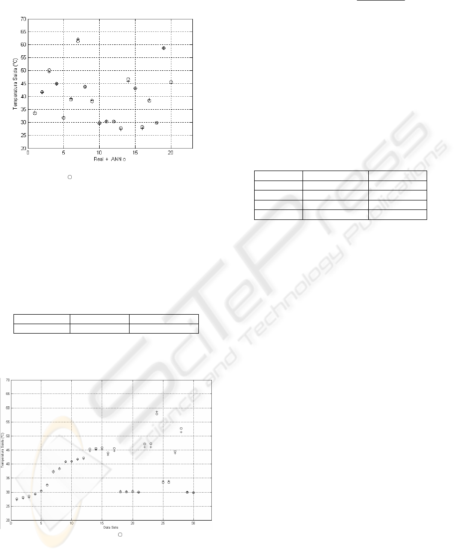
Figure 7 graphically shows the result of training.
Figure 7: Real ( ) and ANN (+) output temperatures.
5.3 Validation of the Neural Network
Table I.2 (append) shows the data set used to
validate the ANN, previously extracted from the
collected data. Table I.2 also shows the output of the
ANN and the errors obtained, compared to the real
output temperature.
Table 2 shows the errors values obtained in the
validation process.
Table 2: Errors from validation process
Min. error (°C) Max. error (°C) Error average (°C)
0.030246 1.359952 0.458544167
Figure 8 graphically shows the results obtained from
the trained and validated net, when operated with the
validation set.
Figure 8: Real (+) and ANN ( ) output temperatures.
5.4 Verification of Results
For the analysis by means of linear regression,
Equation (6) has been used:
G
TT
UFF
ambin
LRe
R
)(
)(
−
−=
ταη
(6)
F
R
(τα)
e
equals 66.662 and F
R
U
L
, 809.89. F
R
corresponds to collector heat removal factor, (τα)
e
, to
transmittance absorptance product and U
L
, to
collector overall loss coefficient. T
in
is the input
water temperature, T
amb
, the ambient temperature
and G, the solar irradiance. Equation (6) calculates
efficiency when linear regression is used.
With the values of the output temperature of the
water, the efficiency of the solar collector can be
calculated. Table 3 shows the comparison between
linear regression and ANN errors in calculating the
efficiency of the solar collector.
Table 3: Comparison between errors.
Eff – Eff ANN (%) Eff – Eff LR (%)
Average 3.124178769 1.864363541
Minimum 0.14650623 0.08587937
Maximum 8.110471201 7.215990429
Std. deviation 2.672893417 1.816157438
6 CONCLUSIONS
In this work, a possible use of ANN to model a solar
collector has been presented. It has been also
presented a technique to build a more representative
training set – the widely used k-means clustering
method. With k-means, a training set composed by
20 data could be used, as shown in Figure 5.
Table 1 shows the results of the training process; the
average error in the output water temperature equals
0.33199 and maximum and minimum errors are,
respectively, 0.92959 and 0.017174. Those results
show the optimal approach of ANN, since the error
recommended by INMETRO (National Institute of
Metrology and Industrial Quality - Brazil) is 1°C.
Efficiency errors, calculated via ANN and linear
regression, are presented in Table 3. Although the
errors obtained via linear regression are lower, ANN
present some advantages on linear regression (e.g.
For new situations with unusual values of entries,
the equation of linear regression may increase the
actual errors values unless it is reformulated, while a
trained net may use its capacity of generalization in
order to maintain the errors values).
Comparing the results of training and validation
processes of a net trained with 631 data (Zárate et al.
2003a), with a training set selected by means of
statistical analysis (Zárate et al. 2003b) and with the
training set of this work, it can be observed that a
better-defined training set may decrease the time
spent in training and may also maintain the capacity
of generalization of the net (Tables 4 and 5).
OPTIMIZATION OF NEURAL NETWORK’S TRAINING SETS VIA CLUSTERING: APPLICATION IN SOLAR
COLLECTOR REPRESENTATION
151

Table 4: Comparing training results.
None
technique
Statistical
analysis
k-means
clustering
Min. error (°C) 0.000035 0.000039 0.017174
Max. error (°C) 1.19 1.021237 0.92959
Error average (°C) 0.15 0.244534 0.33199
N° of iterations
spent in training
7700000 412800 80800
Table 5: Comparing validation results.
None
technique
Statistical
analysis
k-means
clustering
Min. error (°C) 0.02185 0.043265 0.030246
Max. error (°C) 0.70706 1.475292 1.359952
Error average (°C) 0.27365 0.625548 0.458544
ACKNOWLEDGEMENTS
This work has been financially supported by CEMIG
(Energy Company of Minas Gerais - Brazil).
REFERENCES
Morrison, G. L., & Ranatunga, D. B. J. 1980. ‘Transient
response of thermosiphon solar collectors’, Solar
Energy, vol. 24, p. 191.
Huang, B. J. 1984. ‘Similarity theory of solar water heater
with natural circulation’, Solar Energy, vol. 25, p. 105.
Kudish, A. I., Santaura, P., & Beaufort, P. 1985. ‘Direct
measurement and analysis of thermosiphon flow’,
Solar Energy, vol. 35, no. 2, pp. 167-173.
Kalogirou, S. A. 2000. ‘Thermosiphon solar domestic
water heating systems: long term performance
prediction using ANN’, Solar Energy, vol. 69, no. 2,
pp. 167-174.
Kalogirou, S. A., Panteliou S., & Dentsoras A. 1999.
‘Modeling solar domestic water heating systems using
ANN’, Solar Energy, vol. 68, no. 6, pp. 335-342.
Zárate, L. E., Pereira, E. M., Silva, J. P., Vimieiro R.,
Diniz, A. S., & Pires, S. 2003a. Representation of a
solar collector via artificial neural networks. In
Hamza, M. H. ed. International Conference On
Artificial Intelligence And Applications, Benalmádena,
Spain, 8-11 September 2003. IASTED: ACTA Press,
pp. 517-522.
Zárate, L. E., Pereira, E. M., Silva, J. P., Vimieiro, R., &
Diniz, A. S. 2003b. Neural representation of a solar
collector with optimization of training sets
(Unpublished).
Moreira, F., & Roisenberg, M. 2003. Evolutionary
optimization of neural network’s training set:
application in the lymphocytes’ nuclei classification.
In Hamza, M. H. ed. International Conference On
Artificial Intelligence And Applications, Benalmádena,
Spain, 8-11 September 2003. IASTED: ACTA Press,
pp. 358-362.
Duffie, J.A., & Beckman, W. A. 1999. Solar engineering
of thermal processes. 2nd ed. U.S.A.: John Wyley &
Sons, Inc.
Kovács, Z. L. 1996. Redes neurais artificiais, São Paulo,
Brasil: Edição acadêmica, pp. 75-76.
APPEND
Table I.1: Collected data sample.
Tamb Tin Solar Irradiance Tout
25.05 27.17 908.42 33.97
25.91 34.7 1005.68 41.61
23.51 43.42 967.31 49.43
26.26 39.98 761.83 44.73
22.61 25.31 905.41 32.02
23.12 32.82 922.13 39.23
23.75 57.89 958.19 62.21
24.71 38.32 833.93 43.76
25.66 31.65 958.24 38.58
24.49 22.65 872.67 29.46
24.22 23.01 933.09 30.4
23.53 22.83 958.29 30.41
23.96 20.76 768.96 27.28
23.36 39.89 962.33 45.79
25.99 38.11 794.92 43.15
Table I.2: Validation data sets.
Tamb Tin G Tout Tout (ANN) Error
23.83 20.66 755.1 27.17 27.630451 0.460451
24.43 20.97 819.75 27.74 28.14392 0.40392
24.61 21.47 850.02 28.07 28.63377 0.56377
24.44 22.5 860.06 29.27 29.388565 0.118565
24.87 23.72 869.47 30.55 30.365038 0.184962
24.81 25.96 912.59 32.85 32.46125 0.38875
25.31 30.81 932.79 37.52 37.219883 0.300117
25.66 31.65 958.24 38.58 38.304413 0.275587
25.82 33.75 993.54 40.78 40.810246 0.030246
25.85 33.81 996.78 40.86 40.902008 0.042008
25.96 34.65 993.69 41.6 41.772133 0.172133
26.03 34.79 1024.01 41.88 42.176178 0.296178
26.45 37.9 1022.66 44.63 45.445923 0.815923
26.66 38.04 1022.82 45.12 45.592113 0.472113
26.98 38.16 1041 45.27 45.85676 0.58676
26.02 38.18 794.81 43.3 43.93853 0.63853
26.08 39.96 765.05 44.65 45.60505 0.95505
23.77 22.96 924.79 30.32 30.066198 0.253802
24.1 22.98 924.84 30.28 30.099792 0.180208
24.04 23.05 931.81 30.42 30.191616 0.228384
22.76 23.03 907.4 29.93 29.971178 0.041178
23.33 39.98 966.37 46.05 47.142525 1.092525
23.27 40.09 967.81 46.09 47.26527 1.17527
23.74 53.4 983.64 58.6 57.840714 0.759286
25.1 27.13 911.55 33.95 33.501625 0.448375
25.09 27.12 910.06 33.95 33.481182 0.468818
24.65 38.42 849.35 43.85 44.61326 0.76326
24.69 47.01 809.17 51.31 52.669952 1.359952
24.86 23.72 785.5 30.12 29.872047 0.247953
24.96 23.73 770.1 29.83 29.797749 0.032251
ICEIS 2004 - ARTIFICIAL INTELLIGENCE AND DECISION SUPPORT SYSTEMS
152