CONSOLIDATED TREE CONSTRUCTION ALGORITHM:

STRUCTURALLY STEADY TREES

J.M. Pérez, J. Muguerza, O. Arbelaitz, I. Gurrutxaga

Informatika Fakultatea, Basque Country University, po. Box 649, 20080 Donostia, Spain

ywords: decision trees, steadiness, explaining capacity, structural diversity measure

Abstract: This paper presents a new methodology for building decision trees or classification trees (Consolidated

Trees Construction algorithm) that faces up the problem of unsteadiness appearing in the paradigm when

small variations in the training set happen. As a consequence, the understanding of the made classification is

not lost, making this technique different from techniques such as bagging and boosting where the

explanatory feature of the classification disappears. The presented methodology consists on a new meta-

algorithm for building structurally more steady and less complex trees (consolidated trees), so that they

maintain the explaining capacity and they are faster, but, without losing the discriminating capacity. The

meta-algorithm uses C4.5 as base classifier. Besides the meta-algorithm, we propose a measure of the

structural diversity used to analyse the stability of the structural component. This measure gives an

estimation of the heterogeneity in a set of trees from the structural point of view. The obtained results have

been compared with the ones get with C4.5 in some UCI Repository databases and a real application of

customer fidelisation from a company of electrical appliances.

1 INTRODUCTION

Several pattern recognition problems need an

explanation of the made classification together with

a good performance of the classifier related to its

discriminating capacity. Diagnosis in medicine,

fraud detection in different fields, customer

fidelization, resource assignation, etc, are examples

of applications where an explanation of the

classification made becomes as important as the

accuracy of the system. Among the set of

classification techniques that are able to give an

explanation for the classification made, we can find

the decision trees [Quinlan 93]. However,

classification trees have a problem; they are too

sensitive to the sample used in the induction process.

This weakness of decision trees is called

unsteadiness or instability [Dietterich 00a, Chawla el

al 02]. Due to this behaviour, several algorithms for

building classification trees with greater

discriminating capacity and steadiness have been

developed.

Bagging [Breiman 96], boosting [Freund et al 96],

and different variants of them [Chawla el al 02]; are

examples of techniques used to face the problem. All

of them use resampling techniques. Bagging uses a

set of trees induced from different bootstrap

subsamples, extracted from the initial sample

(training set). In the multiple classifier built,

classification is made by simple voting or weighted

voting [Duin et al 00, Bauer et al 99]. When the used

technique is boosting, the different trees are built

sequentially and the patterns are reweigthed

depending on the error made by the preceding

classifier. This makes the next tree in the sequence

concentrate in the hardest zones of the classification

field, so, in the decision boundaries. The final

decision is based on a weighted vote that takes into

account the error estimated during the learning

process of each one of the trees composing the

system.

These techniques obtain improvements in the

behaviour of the global system but they lose the

explaining capacity of the classifier, because in

every case the final classifier is a combination of

different trees with different structures. Our

approximation introduces a new methodology that

brings together both characteristics: stability and

M. Pérez J., Muguerza J., Arbelaitz O. and Gurrutxaga I. (2004).

CONSOLIDATED TREE CONSTRUCTION ALGORITHM: STRUCTURALLY STEADY TREES.

In Proceedings of the Sixth International Conference on Enterprise Information Systems, pages 14-21

DOI: 10.5220/0002602200140021

 SciTePress

explaining capacity. We have developed a new

algorithm for building trees. We denominate the

built trees consolidated trees. This methodology

uses different training subsamples and builds a

single accorded tree among all of them. Every

technique mentioned before to make more stable

classification trees, loses its explanatory component,

because a set of trees with very different structures is

used to make the final decision. Our aim has been to

design a new methodology for building trees that

maintaining the performance of standard

classification trees, reduces the complexity and adds

structural stability to the induced tree. This makes

the explanation related to classification much more

robust and steady, so, less sensible to small changes

in the sample used to build the classifier. In order to

analyse the structural stability of classification trees,

we have defined a diversity measure or distance that

measures how similar or different a set of trees is.

The paper proceeds with the description of our new

methodology for building consolidate trees, Section

2. In Section 3, the structural diversity measure is

introduced, followed in Section 4 by the description

of the data sets and the experimental set-up. The

results of our experimental study are discussed in

section 5. Finally, Section 6 is devoted to summarise

the conclusions and future research.

2 CTC LEARNING ALGORITHM

The tree building methodology we propose,

Consolidated Trees Construction (CTC) algorithm,

is based on resampling techniques. Several training

subsamples are extracted from the original training

set and a single tree is built based on consensus

among the partial trees that are being built from each

subsample. The main difference with bagging,

which makes it radically different, is that the

consensus is achieved in each step of the trees’

building process. The decision about which variable

will be used to make the split in a node is accorded

among the different proposals coming from the trees

(using the base classifier: C4.5 in our case) being

built from the different subsamples. The decision is

made by a voting process. Once the decision about

the variable selected to split the trees is made, all the

trees (each one associated to a different subsample)

are forced to use that variable to make the split. The

process is repeated iteratively until no more

divisions are possible, due to some stop criterion.

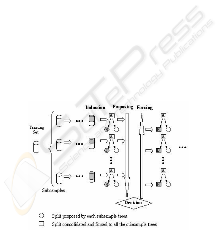
An schema of the algorithm can be found in (Figure

1) and it proceeds the following way:

Figure 1: Consolidation of a node.

CONSOLIDATED TREE CONSTRUCTION ALGORITHM: STRUCTURALLY STEADY TREES

1. Extract a set of subsamples (Number_Samples)

from the original training set using the desired

resampling technique (Resampling_Mode): size

of the subsamples (100%, 75%, 50%, etc; with

regard to the original set’s size), with replacement

or without replacement, stratified or not, etc.

2. The final tree is built node by node in preorder.

Each consolidated node is built the following

way:

a. For each subsample, induce the variable that

would be used to make the split at that level of

the partial tree; in the example (B, F,…,B).

b. Analyse the number of partial trees that

propose to make an split and decide depending

on the established criteria Crit_Split (ex:

simple majority, absolute majority, etc.)

whether to split or not. If the decision is not to

split (a leaf node is created), jump to the next

node to consolidate and go to step 2a.

c. Analyse the number of votes that has the most

voted variable (votes of variable B in Figure 1).

If based on Crit_Variable the variable has not

enough votes, consolidate the node as a leaf

node and go to step 2a. When the number of

votes is enough this variable will be the one

used to split the consolidated node.

d. Decide the branches the node to split will have,

depending on Crit_Branches criteria. If the

variable to split is continuous, determine the

cutting point (ex: using the mean or the median

of the values proposed for that variable). If the

variable to split is discrete, decide the set of

categories for each branch (ex: a branch for

each category, using heuristics such as C4.5’s

subset option, etc.).

e. Force the accorded split (variable and

stratification) in every tree asociated to each

subsample (every partial tree in the example is

forced to make the split with the consolidated

variable B). Jump to next node and go to step

2a.

The different decisions can be made by voting,

weighted voting, etc. Once the consolidated tree has

been built, its behaviour is similar to the one of the

used base classifier. Section 5 will show that the

trees built using this methodology, have similar

discriminating capability (the differences are not

statistically significant) but they are structurally

more steady and less complex. In order to analyse

this second aspect, we have defined the structural

diversity measure that we present in next section.

3 STRUCTURAL DIVERSITY

MEASURE

We will use this section to define the diversity

measure or structural distance, that will allow us to

analyse the stability of the consolidated trees and

compare them to the standard ones. The aim is to be

able to measure the heterogeneity existing in sets of

trees built using each of the methodologies to be

compared. The estimation of the degree of structural

diversity in a group, is made analysing the structural

differences among each possible pair of trees in the

group, and, calculating average values of the

differences obtained.

The defined metric or distance (Structural_Distance,

SD) is based on a vector (M

, M

) with three

values used to compare two trees (T

, T

). Both trees

are looked through in preorder, node by node, and

the corresponding split variables are compared to

know whether they match or not. The three

components are calculated the following way:

• M

: Number of common nodes in T

and T

We understand as common nodes the ones that

being in the same position in both trees, make

the split based on the same variable.

• M

: measures the number of times that

looking through a common branch, a tree

makes a split in a node and the other does not.

Each increment is weighted depending on the

complexity of the subtree beginning in this

node.

• M

: measures the number of times that

looking through a common branch and arriving

to a common node, the variables chosen to

make the split in both trees are different. Each

increment is weighted depending on the

complexity of both subtrees.

The pseudo-code of the algorithm used for

calculating each one of the components of the

proposed measure is in Appendix.

The definitions show that to increase the value of

, the same variable has to appear in the same

node, so that the variable used to make the split has

been chosen at the same level in both trees. Once a

different split appears, the remaining subtrees of the

compared trees have an effect on the value of M

. This is important because in the tree

construction process (top-down), the variables used

to split a node are selected depending on their

statistical importance (entropy, p-value, ...). As a

consequence, this measure of similarity/diversity

takes also into account when making the

ICEIS 2004 - ARTIFICIAL INTELLIGENCE AND DECISION SUPPORT SYSTEMS

comparison, the statistical importance each tree has

given to each of the independent variables.

We have defined two measures, M

and M

, because

indicates higher diversity level among the trees

than M

does, and we think that it is important to

differentiate both cases.

Evidently, when greater is the first component and

smaller the two others, more homogeneous is the set

of trees used to calculate the values.

In order to calculate the diversity in the set of trees

we estimate the mean of the vector:

2,1,0

),(

)1(

)(

−

∑

−

xwith

TTSD

TSD

set

mean

(1)

Once the vector has been obtained, the comparison

between groups can be done at vector level or at

scalar level making any combination of the different

components depending on the importance we want

to give to each of the measures get.

In this case we define a scalar measure

(%Common

mean

) based in three percentages

calculated from the three components normalised in

respect to the sum of the number of nodes of the two

trees compared. The scalar is computed with a lineal

combination of the three percentages with the vector

of weights (1,-1,-1). In this experimentation we

don’t take into account the different level of

importance of the two last components. If the scalar

measure is positive, the compared trees are more

similar than different among them, and, when the

value is negative the common part of the trees is

smaller than the different one. The range of values

the scalar can take is between –100 and +100. This

measure allows the comparison of groups of trees

with different complexities (at the structural level),

because the components are normalised in respect to

the number of nodes of the comparison.

4 EXPERIMENTATION

Six databases of real applications have been used for

the experimentation. Most of them belong to the

well known UCI Repository benchmark [Blake et al

98], widely used in the scientific community. Table

1 shows the characteristics of the databases used in

the comparison. The last database is a real data

applications from our environment, and does not

belong to UCI. The data set called Faithful is centred

in the electrical appliance’s sector. In this case, we

try to analyse the profile of the customers during the

time, so that a classification related to their fidelity

to the brand can be done. This will allow the

company to follow different strategies to try to

increment the number of customers that are faithful

to the brand, so that the sales increase. In this kind of

applications is very important to use a system that

provides information about the factors taking part in

the classification (the explanation), because it is

nearly more important to analyse and explain why a

customer is or is not faithful, than the own

categorisation of the customer. This is the

information that will help the corresponding

department to make good decisions.

Table 1: Description of experimental domains

Domain

N. of patterns N. of features N. of classes

Breast cancer W 699 10 2

Heart disease C 303 13 2

Hypothyroid 3163 25 2

Lymphography 148 18 4

Segment 210 19 7

Faithful 24507 49 2

The CTC methodology has been compared to the

C4.5 tree building algorithm Release 8 of Quinlan

[Quinlan 93], using the default parameters’ settings.

The methodology used for the experimentation

[Hastie et al 01] is a 10-fold stratified cross

validation. Cross validation is repeated five times

using a different random reordering of the examples

in the data set. This methodology has given us the

option to compare 5 times groups of 10 trees CTC

and C4.5 in both senses the structural point of view

and the discriminating capacity (50 executions for

each instance of the analysed parameters). In each

run we have calculated the average error and its

standard deviation, together with the SD

mean

set

) of

each of the groups of trees and the values

Comp

mean

(estimated as the number of internal nodes

of the tree) and %Common

mean

(explained in Section

3).

In order to evaluate the structural improvement

achieved in a given domain by using the algorithm

CTC compared to the algorithm C4.5, we have

calculated, (%Comm

CTC

-%Comm

C4.5

)/%Comm

C4.5

the relative improvement.

For every result we have tested the statistical

significance [Dietterich 98, Dietterich 00] of the

differences of the results obtained with the two

algorithms using the paired t-test (with significance

level of 95%).

CONSOLIDATED TREE CONSTRUCTION ALGORITHM: STRUCTURALLY STEADY TREES

5 RESULTS

We have analysed several parameters of the CTC

meta-algorithm. The ranges of the different

parameters analysed are:

1. Number_Samples: 3, 5, 10, 20, 30, 40, 50, 75,

100, 125, 150, 200. The obtained results show

that 10 is the minimum number of samples to

achieve satisfactory results with CTC. So, the

average results presented in this section do not

take into account the values 3 and 5, except for

Faithful where due to the size of the database the

study has been done from 3 to 40 subsamples.

2. Resampling_Mode: due to the importance of the

diversity of the subsamples used to build a

classifier [Skurichina et al 00], different options

have been proved (samples of size 50% and 75%

of the original training set drawn without

replacement, and bootstrap samples). The best

results have been obtained with the 75% (results

shown in the paper), probably because this is the

case where each subsample has larger amount of

information of the original sample.

3. Crit_Split and Crit_Variable: simple majority

among the Number_Samples for both. The

possibility of introducing thresholds to these

criteria has not been considered in this paper

because the comparison of our consolidated trees

(CTC) with the simple classification trees C4.5

has been done pruning the trees with the pruning

algorithm of the C4.5 Release 8 software. The

pruning has been done in order to obtain two

systems with similar complexity level (the same

zone in the learning curve) and also to be able to

make the structural comparison with similar

development conditions for all trees. We can not

forget that developing too much a classification

tree leads to a greater probability of overtraining

and on the other hand, the fact that a variable

appears in the tree is less significant because the

system takes into account very specific details of

the training set.

4. Crit_Branches: the selection of the new branches

to be created when the variables are continuous

has been made based on the median.

Experimentation with the mean has also been

done, but the results were worse, probably

because this measure has smaller stability. When

the variables were discrete we have not used the

subset option of C4.5 and as many branches as

categories has the variable selected to make the

split have been proposed.

Table 2: Error and complexity comparison among C4.5 and CTC. The best values related to Number_Samples in each data

set are shown

C4.5 CTC (ERR

MIN

) CTC (COMP

MIN

)

Err Comp Err R.Dif Comp R.Dif N_S Err R.Dif Comp R.Dif N_S

Breast-W 5.63 3.16 5.40 -4.12 3.11 -1.41 125 5.49 -2.49 3.04 -3.52 30

Heart-C 23.96 15.11 22.85 -4.61 13.51 -10.59 20 22.92 -4.35 13.20 -12.65 30

Hypo 0.71 5.38 0.72 0.56 4.51 -16.12 20 0.72 0.84 4.40 -18.18 30

Lymph 20.44 8.84 19.65 -3.88 9.24 4.52 30 19.93 -2.51 9.09 2.76 40

Segment 13.61 11.71 11.52 -15.31 13.82 18.03 50 13.51 -0.75 12.64 7.97 10

Faithful 1.48 39.47 1.48 -0.13 32.44 -17.79 20 1.50 0.94 28.56 -27.65 05

Average

10.97 13.94 10.27 -4.58 12.77 -3.89 10.68 -1.38 11.82 -8.54

Table 2 shows the results related to error (Err) and

complexity (Comp) for the different data sets. The

comparison among C4.5 and CTC we present in the

table has been calculated using the best value of the

parameter Number_Samples (N_S) for CTC in order

to minimise the error or the complexity of the

classifier. The relative differences among the two

algorithms (R.Dif) are also presented, for both

parameters, the error and the complexity. The last

row shows the mean of the results obtained with the

two algorithms, for the different domains. It can be

observed that in average, the CTC algorithm obtains

a relative improvement in the error of 4.58%. In this

case, when talking about the complexity of the

generated trees, the relative improvement is 3.89%.

Even when the best Number_Samples for

minimising the complexity has been selected, the

CTC has smaller errors than the C4.5, being the

improvement 1.38%. The relative complexity

reduction obtained in this case is 8.54%. In the

larger database we have used (Faithful), where the

reduction of the complexity becomes more

important, the obtained improvement is 27.65%.

This reduction is statistically significant for every

value of the parameter Number_Samples.

To confirm the robustness of the algorithm when the

parameter Number_Samples is changed, Table 3 (left

side) shows the average values of the error and the

complexity obtained with all the analysed values for

that parameter.

ICEIS 2004 - ARTIFICIAL INTELLIGENCE AND DECISION SUPPORT SYSTEMS

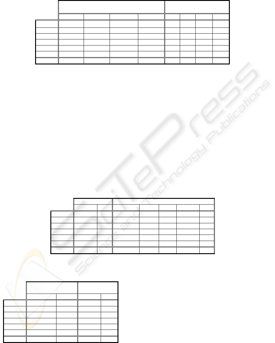
Table 3: Average results of the error and the complexity in CTC taking into account the whole range of N_S (left side) and

for N_S=30 (right side)

CTC

(Average N_S=10,20,30,40,50,75,100,125,150,200)

CTC

N_S=30

Err R.Dif Comp R.Dif Err R.Dif

Comp

Dif

Breast-W

5.56 -1.21 3.09 -2.11 5.49 -2.49 3.04 -3.52

Heart-C 23.43 -2.21 13.84 -8.41 22.92

-4.35 13.20 -12.65

Hypo 0.73 2.30 4.65 -13.60 0.72 0.84 4.40 -18.18

Lymph 20.03 -2.01 9.18 3.74 19.65

-3.88 9.24 4.52

Segment 12.42 -8.70 14.08 20.23 13.13

-3.48 13.47 14.99

Faithful 1.49 0.84 30.03 -23.92 1.49 0.67 29.53 -25.17

Average

10.61 -1.83 12.48 -4.01 10.57

-2.11 12.15 -6.67

It can be observed that a relative improvement of

1.83% in the error is maintained and the complexity

improves in a 4.01%. If we would like to tune the

parameter in order to optimise the error/complexity

trade off in the analysed domains, the results address

us to N_S=30. The results for N_S=30 appear in

Table 3 (right side). They do not differ substantially

from the results obtained finding in each domain the

best value for Number_Samples. The CTC maintains

its improvement if compared to C4.5 in both cases.

If we analyse the statistical significance of the

differences among the two algorithms, we won’t

find significant differences in the error parameter for

none of the values of Number_Samples. However,

when analysing the complexity significant

differences in favour of CTC are found in three of

the six databases (Heart-C, Hypo, Faithful).

Regarding to the structural stability of the trees

obtained with each algorithm, and taking into

account the metric presented in Section 3, Table 4

shows that except in one of the databases (Lymph),

the trees built using CTC algorithm, are more similar

among them than the ones generated with C4.5. This

means that the induction mechanism is able to

extract more information about the explanation of

the classification, and besides, in a more steady way.

The improvement is in average of 16.82%, and, the

differences are statistically significant in every case

where better results are obtained.

Table 4: Comparison of C4.5 and CTC related to the structural diversity measure, using the best value of Number_Samples

in each domain

C4.5 CTC (%COMM

MIN

)

%Comm

Err %Comm R.Dif Err R.Dif N_S

Breast-W

56.99 5.63 65.89 15.62 5.49 -2.49 30

Heart-C -59.01 23.96

-57.06 3.30 23.16 -3.32 150

Hypo 27.99 0.71 41.11 46.90 0.73 2.53 75

Lymph -27.72 20.44

-35.50 -28.08 20.18 -1.25 75

Segment -67.09 13.61

-36.19 46.06 12.76 -6.26 20

Faithful -57.95 1.48 -48.01 17.15 1.50 0.94 05

Average

-21.13 10.97

-11.63 16.82 10.64 -1.64

Table 5: Average results of the structural metric in the

CTC algorithm. The whole range of N_S is taken into

account in left side and N_S=30 in right side

CTC

(Average N_S=10..200)

CTC

N_S=30

%Comm R.Dif %Comm

R.Dif

Breast-W

60.51 6.19 65.89 15.62

Heart-C -61.10 -3.53 -58.57 0.75

Hypo 35.15 25.60 37.14 32.69

Lymph -36.71 -32.43 -36.76 -32.62

Segment -47.16 29.70 -43.33 35.41

Faithful -50.71 12.49 -50.94 12.09

Average

-16.67 6.33 -14.43 10.66

Table 5 shows in the left side the mean of the

differences in the structural metric of both

algorithms, for all the experimented values with

parameter Number_Samples. The average value

favours CTC, and, we should not forget that the

error also favours it. This proves again the stability

of the meta-algorithm in respect to the tuning of the

parameter Number_Samples.

The same table, right side, presents results of the

structural diversity among both algorithms, when

N_S=30. The results in this case are near the optimal

results we found and better than the average results

obtained (left side). As a consequence we can ensure

that the influence of the parameter Number_Samples

in the final result is not critical in any of the

analysed criteria.

CONSOLIDATED TREE CONSTRUCTION ALGORITHM: STRUCTURALLY STEADY TREES

6 CONCLUSIONS AND FURTHER

WORK

A new algorithm to build classification trees that are

structurally more steady and with smaller

complexity level has been presented (Consolidated

Trees Construction, CTC). This algorithm achieves

and even improves the discriminating capacity of

C4.5. The proposed algorithm maintains the

explanatory feature of the classification and this is

very important in many real life’s domains. The

algorithm builds trees that reduce the error rate and

the complexity of the classifier if compared to the

C4.5.

Besides, and to prove the goodness and the stability

of the explanation related to the classification, a

measure of the structural diversity of two trees is

proposed. This measure analyses the stability of the

variables and their statistical importance (level

where they appear in the tree). The measure allows

the analysis of the heterogeneity of a set of trees

from the structural or explanatory point of view.

In this paper we have proven that for the analysed

domains, the CTC is able to extract more

information about the explanation of the

classification, and, in a more steady way. The

differences are statistically significant in most of the

analysed domains.

On the other hand, the stability of the meta-

algorithm when varying the parameter

Number_Samples has been proved; N_S=30 is an

adequate value for all the databases used in the

experimentation.

The first work to do in the future is to enlarge the set

of domains analysed. We are also thinking on

experimenting with other possibilities for the

parameter Resampling_Mode (different amount of

information or variability of the subsamples) as

further work.

Other interesting possibility is to generate new

subsamples dynamically, during the building process

of the CTC, where the probability of selecting each

of the cases is modified based on the error (similar

to boosting).

We are also analysing a possibility where the own

meta-algorithm builds trees that do not need to be

pruned. With this aim, we would make a tuning of

the parameters Crit_Split and Crit_Variable, so that

the generated trees are situated in a better point of

the learning curve and the computation load of the

training is minimised. Heuristic techniques for the

stratification of the discrete variables can also be

studied in order to build trees with greater

explaining capacity.

This methodology can be very useful when

resampling is compulsory (large databases, class

imbalance, ...).

APENDIX

int CalculateSD (Tree Ti, Tree Tj,

int VMetric[])

{

if ((Ti->NodeType != LEAF) &&

(Tj->NodeType != LEAF))

if (Ti->Variable == Tj->Variable)

{VMetric[0]++;

if (Ti->Forks != Tj->Forks)

return (–1);

ForEach(k,1, Ti->Forks)

CalculateSD (Ti->Branch[k],

Tj->Branch[k],VMetric);

}

else //different division variables

{Vmetric[2]+=

CalcNumberDescendents(Ti);

Vmetric[2]+=

CalcNumberDescendents(Tj);

return (0);

}

else

if ((Ti->NodeType == LEAF) &&

(Tj->NodeType == LEAF))

return (0);

else

if (Ti->NodeType = LEAF)

{Vmetric[1]+=

CalcNumberDescendents(Tj);

return (0);

}

else

{Vmetric[1]+=

CalcNumberDescendents(Ti);

return (0);

}

return (–1);

}

ICEIS 2004 - ARTIFICIAL INTELLIGENCE AND DECISION SUPPORT SYSTEMS

ACKNOWLEDGEMENTS

The work described in this paper was partly done

under the University of Basque County / Euskal

Herriko Unibertsitatea (UPV/EHU) project: 1/UPV

00139.226-T-14882/2002.

We would like to thank the company Fagor

Electrodomesticos, S. COOP. for permitting us the

use, in this work, of their data (Faithful) obtained

through the project BETIKO.

The lymphography domain was obtained from the

University Medical Centre, Institute of Oncology,

Ljubljana, Yugoslavia. Thanks go to M. Zwitter and

M. Soklic for providing the data.

REFERENCES

Quinlan J. R., 1993. C4.5: Programs for Machine

Learning. Morgan Kaufmann Publishers Inc.(eds), San

Mateo, California.

Dietterich T.G., 2000. Ensemble Methods in Machine

Learning. Lecture Notes in Computer Science, Vol.

1857. Multiple Classifier Systems: Proc. 1st. Inter.

Workshop, MCS, Cagliari, Italy, 1-15

Chawla N.V., Hall L.O., Bowyer K.W., Moore Jr.,

Kegelmeyer W.P., 2002. Distributed Pasting of Small

Votes. Lecture Notes in Computer Science Vol. 2364.

Multiple Classifier Systems: Proc. 3th. Inter.

Workshop, MCS, Cagliari, Italy, 52-61

Breiman L., 1996. Bagging Predictors. Machine Learning,

24, 123-140

Freund, Y., Schapire, R. E., 1996. Experiments with a

New Boosting Algorithm. Proceedings of the 13th

International Conference on Machine Learning, 148-

156

Duin R.P.W, Tax D.M.J., 2000. Experiments with

Classifier Combining Rules. Lecture Notes in

Computer Science 1857. Multiple Classifier Systems:

Proc. 1st. Inter. Workshop, MCS, Cagliari, Italy, 16-

Bauer E., Kohavi R., 1999. An Empirical Comparison of

Voting Classification Algorithms: Bagging, Boosting,

and Variants. Machine Learning, 36, 105-139

Blake, C.L., Merz, C.J., 1998. UCI Repository of Machine

Learning Databases. University of California, Irvine,

Dept. of Information and Computer Sciences

http://www.ics.uci.edu/~mlearn/MLRepository.html

Hastie T., Tibshirani R. Friedman J., 2001. The Elements

of Statistical Learning. Springer-Verlang (es). ISBN:

0-387-95284-5

Dietterich T.G., 1998. Approximate Statistical Tests for

Comparing Supervised Classification Learning

Algorithms. Neural Computation, 10, 7, 1895-1924

Dietterich T.G., 2000. An Experimental Comparison of

Three Methods for Constructing Ensembles of

Decision Trees: Bagging, Boosting, and

Randomization. Machine Learning, 40, 139-157

Skurichina M., Kuncheva L.I., Duin R.P.W., 2002.

Bagging and Boosting for the Nearest Mean Classifier:

Effects of Sample Size on Diversity and Accuracy.

Lecture Notes in Computer Science 2364. Multiple

Classifier Systems: Proc. 3th. Inter. Workshop, MCS,

Cagliari, Italy, 62-71

CONSOLIDATED TREE CONSTRUCTION ALGORITHM: STRUCTURALLY STEADY TREES