ARTIFICIAL INTELLIGENCE REPRESENTATIONS OF MULTI-

MODEL BASED CONTROLLERS

Asier Ibeas, Manuel de la Sen

Instituto de Investigación y Desarrollo de Procesos, Facultad de Ciencia y Tecnología

Universidad del País Vasco, Apdo. 644, 48080 Bilbao, Spain

Keywords: Multimodel control, artificial intelligence, neural networks, genetic algorithms, fuzzy logic, switching.

Abstract: This paper develops a representation of multi-model based controllers by using artificial intelligence typical

structures. These structures will be neural networks, genetic algorithms and fuzzy logic. The interpretation

of multimodel controllers in an artificial intelligence frame will allow the application of each specific

technique to the design of multimodel based controllers. A method for synthesizing multimodel based

neural network controllers from already designed single model based ones is presented. Some applications

of the genetic algorithms and fuzzy logic to multimodel controller design are also proposed.

1 INTRODUCTION

Multi-model based controllers have been broadly

studied during the last years (Narendra et al, 1997,

Gregorcic et al, 2001, Ibeas et al, 2003). This kind of

control architecture allows to design intelligent

control systems able to modify their behavior

according to the characteristics of a changing

environment or operation point. This intelligent

behavior, allows the stability and improvement of

the closed-loop output for complex systems. Thus, a

general multimodel based control scheme is formed

by a set of different plant models running in parallel.

These models, which may be fixed (Narendra et al,

1994) or adaptive (Ibeas et al, 2003), are different

one from each other in what it is concerned with its

structure or its parameter values. Thus, each one

contains different characteristics of the controlled

process. Moreover, a higher level switching

structure between the various models chooses at

each time the model which will be used to calculate

the control law at that time instant. The switching

structure chooses the control model according to a

performance index for the closed-loop system. Thus,

the switching law acts as a supervisor of the system

behavior. The structure and operation of the

switching law has been studied from an artificial

intelligence point of view in an expert systems

context (De la Sen et al, 2002). However,

multimodel structures itself, have always been

modeled in a classical control theory frame

(Narendra et al, 1997). This paper proposes a

possible interpretation of multimodel schemes in an

artificial intelligence frame. The artificial

intelligence structures chosen for such a goal have

been, artificial neural networks (ANN), genetic

algorithms (GA) and fuzzy logic. This interpretation

will allows the use of specific characteristics of each

one to the design of improved multimodel control

schemes. Thus, a method for synthesizing

multimodel-based neural network controllers from

pre-designed single model ones is proposed. Also,

some applications of genetic algorithms and fuzzy

logic to multimodel control design are presented. An

adaptive, being more general than that related to the

use of fixed models, formalism is used for making

the interpretation.

2 BASIC MULTIESTIMATION

SCHEME

In this Section, a brief description on the

multiestimation scheme used for discussion is

presented. It has been considered the adaptive case

since the fixed case is included in this as a particular

case. The aim is to design a multimodel control for

the discrete (the continuos case can be treated in the

165

Ibeas A. and de la Sen M. (2004).

ARTIFICIAL INTELLIGENCE REPRESENTATIONS OF MULTI-MODEL BASED CONTROLLERS.

In Proceedings of the Sixth International Conference on Enterpr ise Information Systems, pages 165-171

DOI: 10.5220/0002597801650171

 SciTePress

same way) time invariant linear SISO plant

described by:

() ()

qy Bqu

−−

= (1)

where

u and

y are the input and the output

sequences respectively,

−

is the one-step delay

operator,

q is the one-step forward operator and

112

()1

qaqaqaq

−−− −

=+ + + +K (2.1)

()

qbbq bq

−−−

=+ ++K (2.2)

with

≥ . The above Equations (1-2) represent a

linear difference equation which is usually written in

adaptive control as the inner product of two vectors

θθ

== (3)

[]

12 1

k k kn k k km

yy yuu u

−− − − −

=− − −LL

being the so called regressor and

[]

12 01

aabbb

= LL

symbolising the true plant parameter vector (Ibeas et

al, 2003). If the true plant parameter vector is

unknown, parameter estimation has to be used.

Thus, an estimated parameter vector

is considered

at each sample

k. This estimated vector is used for

control calculations at each sample. If this estimated

vector is far away from the real plant parameter

vector, then the transient response will have large

deviations from the desired output resulting in a bad

performance. This fact motivates to consider a set of

estimation algorithms running in parallel, each one

with its own estimated parameter vector

()

(1) (2)

ˆˆ ˆ

, ,...,

kk k

θθ θ

, where

is the number of total

estimators. Each estimated vector is updated at each

sample according to input and output measurements

of the plant. The multiestimation scheme block

diagram is displayed in Figure 1. A switching logic

between the various estimation algorithms chooses

the estimated vector that achieves the best system

behavior improvement according to a prescribed

performance index

()

iN≤≤ . The switching

law must respect a minimum

dwell or residence time

between consecutive switchings in order to

guarantee closed-loop stability.

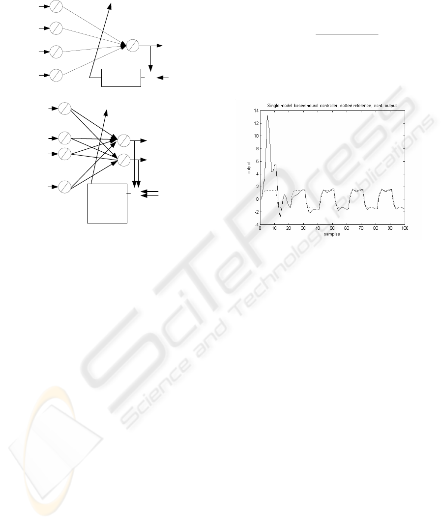
Figure 1: Basic Multiestimation Scheme

A complete discussion of the stability issues is

available in (Ibeas et al, 2003). In the next sections

an artificial intelligence representation of the above

multiestimation scheme is given for various typical

artificial intelligence structures (Da Ruan, 1997).

3 ARTIFICIAL NEURAL

NETWORKS

In this section, an artificial neural network (ANN)

representation is developed for the above

multiestimation based control scheme (Fausett,

1998). In (Etxebarria, 1994), a two layered ANN is

presented for a discrete time single adaptive control.

The difference Equation (1)-(2) is implemented for

estimation purposes by the ANN displayed in Figure

2, where the activation functions are linear for all

neurons. The ANN output can be written as:

,1,

ik k i n j k k j k

ywy wuw

−++−

=+ =

∑∑

(4)

where:

1, 2, ,

kk nmk

www w

⎡

⎤

⎣

⎦

and

is the so called regressor. Comparing the

above Equation (4) with Equation (3), it can be

observed that network weights

represents the

estimated plant parameters. Networks weights (or

plant parameters) are updated by using the well

known

Widrow-Hoff rule for single-output multiple-

input ANN:

()

kkk

εϕϕ

−

−−

−

(5)

where

denotes ANN output while

denotes real

measured plant output and

> ,

()

0,2

∈ ,

(Etxebarria, 1994). Thus, network weights are

updating by comparing the network output with the

real plant output (which it is the target value). Then,

the estimated weights vector (which is the estimated

ICEIS 2004 - ARTIFICIAL INTELLIGENCE AND DECISION SUPPORT SYSTEMS

166

plant parameters vector) is used for controller design

purposes.

−

⊗

Widrow-Hoff

Rule

−

nmk

Figure 2: Single neural network estimator

(1)

(2)

−

⊗

Multiple

output

W idrow-Hoff

Rule

−

−+

−

Figure 3: Multiestimation neural network

Now, the multiestimation scheme presented in

Section 2 can be represented by increasing the

number of neurons in the output layer to a number

of neurons equal to the number of different

estimators used in the multiestimation scheme

. Since

the output layer has one neuron in this case, a

multiestimation scheme with

estimators running

in parallel will have

neurons in its output layer

as the Figure 3 displays for the case of two

estimators. Hence, the number of connections and

weights between neurons is increased. Thus, the

proposed ANN is an structure containing itself the

estimated parameter vectors (which are

represented by the corresponding weights). The

target vector (with which the ANN is trained) is

defined in this case by repeating the original target

value as many times as the number of estimators

used. If the original target value was the real

measured plant output,

, in the case with two

estimators, the new target vector is defined by:

[]

y=y

while in the general case with

estimators, it is:

kk k

⎡⎤

⎢⎥

⎣⎦

144

443

The switching logic compares each output of the

ANN with the real plat output and chooses the set of

weights associate with the best estimated output in

order to calculate the control law. The training rule

is the generalization of the above

Widrow-Hoff

single output training rule (5) to the multiple output

case:

()

,,1

kkjk

ij k ij k

αϕ

εϕϕ

−

−−

−

(6)

where

−

stands for the j-th component of the

vector

−

. Note that the updating law for the

estimated parameters vectors (network weights) is

formulated for the multiple output ANN as a unique

Figure 4: Single model based output

identity. In the following, a simulation example is

presented containing two estimation algorithms and

the above training rule. The switching logic is

assumed to respect a minimum residence time

between successive switchings in order to guarantee

closed-loop stability (Ibeas et al, 2003). The discrete

plant has the real plant parameter vector

[]

.9 0.73 0.195 1 0.6 0.087

=− − − and

the reference model is:

[]

.6 0.11 0.006 1 0.32 0.025

=− − −

while the estimators are initialised by the following

estimated parameter vectors (or network weights) :

[]

(1)

0.5 0.25 0.5 0.79 0.5 0.08

=− − −

[]

(2)

1.5 0.7 0.2 0.9 0.5 0.08

=−−−

It is taken

0.001

= and

= . The input signal is a

unity square wave with a 20 samples period. The

residence time is 2 samples and the performance

index to decide switches is

()

() ()

()

iki

Jk yy

−

=−

∑

(7)

with the forgetting factor

0.95

= . The single

adaptive control scheme is initialised with the first

estimator. Simulations are showed in Figures (4-6).

ARTIFICIAL INTELLIGENCE REPRESENTATIONS OF MULTI-MODEL BASED CONTROLLERS

167

Figure 5: Multimodel based neural controller.

Figure 6: Switching map for the multimodel ANN.

It is showed that the system improves its behaviour

by using the best weight set at each time (respecting

the residence time constraint) Figures (4-5). The

switching map

illustrating the switching process

between both set of weights (parameters) is showed

in Figure 6. The above idea can be extended to the

most general case in which the ANN has a number

of layers greater than two and a number of neurons

in the output layer greater than one. Thus, the

following rule is proposed in order to obtain

multimodel based ANN controllers from a pre-

designed ANN single model one. Suppose that the

single model ANN has

layers and

neurons

in its output layer. Now, define a new ANN for the

multimodel structure as an ANN with the same

number of layers as the original one and a number of

neurons in the output layer equal to

NN=

where

is the number of estimators considered.

The target vector in this case is built by repeating the

original target vector (from the single model ANN)

as many times as the number of estimators

considered. The switching logic acts as an intelligent

supervisor deciding the set of weights that will be

used for control purposes. In such an easy way, the

multimodel structure can be integrated with

conventional neural network based controllers in

order to obtain more general ANN based multimodel

{

inputs

MMM

}

N −

}

outputs

(1)

out

(1)

out

(2)

out

(2)

out

()

out

()

out

Figure 7: General multimodel ANN scheme.

structures. The training rule is the same as in the first

ANN, extended to the new weights associated to

new connections. The general multimodel neural

network scheme is displayed in Figure 7.

4 GENETIC ALGORITHMS

In this Section, a genetic algorithm representation is

given for multiestimation based control schemes.

Genetic algorithms are usually used as optimisation

tools in complex problems (Beyers, 1998). The key

idea is to use the natural selection and the genetics

to obtain at each generation more accurate solutions

to an original complex problem. First, a codification

for the solutions for the proposed problem is

decided. The codification process consists of

deciding how the information about our problem has

to be managed by the genetic algorithm. The

codification may be formed by binary (formed by

1’s and 0’s) or numeric (natural, real,…) vectors.

These vectors are called chromosomes in the GA

context. In the multiestimation case, the

chromosomes will be vectors of real components

containing the plant parameter values. The best

vector is that for which the estimated output

(associated to that parameter vector) is closer to the

real plant output. A general description of a genetic

algorithm is given by the Figure 8. In the first step,

there exists an initial set of vectors uniformly

distributed over the possible parameter space.

ICEIS 2004 - ARTIFICIAL INTELLIGENCE AND DECISION SUPPORT SYSTEMS

168

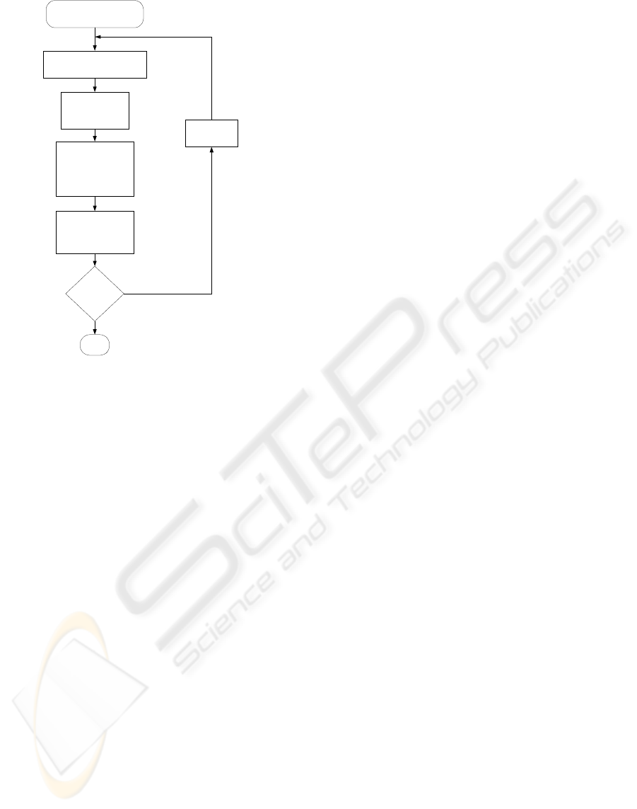
Initial Population

(Initialization of the estimates vectors)

Evaluation of each individual fitness

(Performance index for each estimator)

Selection of the parents

(Slection of a subset of

potentially estimator

algorithms)

Generate the offsprings by

applying various genetic

operators, croos over,

mutation, ...

(Obtain the new vector from

the particular estimation

algorithm used)

Replace the population with

the new offsprings

(The new estimates vector are

used for control an supervision

purpouses)

Finish?

End

Next generation

(Next sample, step)

YES

Figure 8: General structure of a genetic algorithm

This is a typical assumption in the adaptive control

problem, the existence of a convex and compact

subset of the parameter space where the real plant

parameter vector is assumed to belong to. Once the

GA is initialised it starts running. First, one of the

above vectors is chosen in order to generate the

control law. The selection is made according to a

performance index which evaluates the quality of

each vector (in the first step the choice may be

arbitrarily). The unique requirements about the

performance index (in a GA context) are that it must

be nonnegative and monotonically increasing with

quality, i.e., the better vector is that which has the

greater performance index. Then, the parameter

estimated vector are modified by applying some

modification rules. The modification rules may

depend on the value of the performance index

associate with each vector. In GA terms, these

modification rules are called, selection, crossover

and mutation. The adaptive counterpart is the

updating rule for the estimation algorithms such as

the least squares one or any of its variants for

example. Once the new chromosomes are obtained,

the algorithm evaluates the quality of each new

vector in order to obtain the best one and the process

is repeated so on. Note that the GA representation

allows a broad class of modification rules for the

estimated vectors which may not be driven by a

classical parameter updating equation. Furthermore,

the number of different models (the number of

chromosomes) may not be constant during the

system operation. This suggests the following

interesting idea for multimodel based controllers. If

the system detects that with a reduced number of

models an acceptable system behaviour is achieved,

then it may suppress some of the models

(chromosomes) in order to prune unnecessary

computations. Thus, the multiple models are

classified into priority sets in such a way that models

with a similar performance belong to the same set

(according to some performance criteria, for

example, all models with performance index inside a

prescribed range belong to the same set). Thus, the

sets associated to models with the worst

performance may be pawn from the GA process

while those sets containing the most accurate models

may be recompensed by increasing the number of

models inside them. Thus, from a general uniformly

spaced different models, the system is able to obtain

an improved number of models achieving an

acceptable system performance.

5 FUZZY LOGIC APPROACH

In this Section, a fuzzy logic approach is given for

multiestimation based control schemes. As it is

known, fuzzy set theory is a generalization of the

classical set theory (Tilli, 1992). It allows a class of

objects with a continuum grade of membership.

Such a set is characterised by a membership

(characteristic) function which assigns to each object

its grade of membership ranging from one to zero.

The classical set theory operations are extended to

the fuzzy case as well. Inference relations over fuzzy

set objects define the so called fuzzy logic. In the

multiestimation scheme presented in Section 2, an

estimated parameter vector is chosen from a set of

parameter estimated vectors to parameterise the

adaptive controller at each sampling time. However,

instead of choosing a single estimated vector, it is

also possible to define a combined estimated vector:

()

(1) (2)

1, 2, ,

ˆˆ ˆ ˆ

...

kkk kk Nkk

θαθ αθ αθ

=+ ++ (8)

where

≤≤,

N≤≤

and

k∀≥ . This linear

combination (8), is convex in the sense that

∑

k∀≥ . In the standard cases (considered

above and in (Ibeas et al, 2003)), only one

coefficient

is different to zero and equal to

unity. However, it is also possible to let each

coefficient

take a value between one to zero.

Then, we can interpret each one as a membership

ARTIFICIAL INTELLIGENCE REPRESENTATIONS OF MULTI-MODEL BASED CONTROLLERS

169

function of the combined estimated vector

to the

corresponding estimation algorithm with vector

()

The following membership function is proposed in

order to clarify the interpretation:

()

(

)

−

∑

(9)

where the

()

symbolizes the performance indexes

for evaluating the quality of each estimation scheme.

A bigger performance index for an estimation

algorithm leads to a less membership function for

the combined estimated vector to the corresponding

estimation algorithm associate estimated vector. The

fuzzy logic approach allows that the membership

functions may be determined by linguistic rules as

If f(condition1, condition2,…,conditionN) is true

Then modify membership functions as (… rules…)

where f(·) is a logical function of its arguments. As

an example, it may be possible to avoid control

singularities associated with pole-zero cancellations

0 10 20 30 40 50 60 70 80 90 100

-2

-1

samples

output

Desired output(dashed), single adaptive (dotted) and combined adaptive (solid)

Figure 9: Comparison between classical and combined

schemes.

in pole placement control algorithms. Given a set of

estimated parameter vectors, add another vector (or

vectors) to the set. This vector (or vectors, which

may be fixed or updated at each sample) represents

coprime pole-zero polynomials. If the system is near

a control singularity (condition that can be detected

with a prescribed threshold by using the determinant

of the Sylvester matrix for example), then modify

membership functions in such a way that

singularities in the control law are avoided.

Membership functions are modified in order to make

more representative the coprime vectors in such a

way that the combined estimated vector remains

coprime. Thus, linguistic rules for specifying the

system behavior can be included in the system

operation increasing the way in which multimodel

based controllers can be designed. Each estimated

parameter vector is updated according to its

corresponding estimation scheme. The updating

the membership functions must respect a minimum

residence time in order to guarantee closed-loop

stability. The following simulations show the

usefulness of the proposed scheme. The plant, the

input signal and the performance index used in (9)

are the same as in the ANN example (7). The

estimation algorithm is of least squares type. The

residence time is 5 samples. There are five

estimators initialized by:

[]

(1)

0.50.2 0.50.79 0.350.082

=− − −

[]

(2)

1 0.4 0.4 0.9 0.45 0.084

=− − −

[]

(3)

1.5 0.6 0.3 1 0.55 0.086

=− − −

[]

(4)

2 0.8 0.2 1.2 0.65 0.088

=− − −

[]

(5)

2.5 1 0.15 1.5 0.75 0.088

=− − −

The initial values for the membership functions are:

[]

515151515

= and they are updated

by Equation (9) respecting the residence time

constraint. The single adaptive control scheme is

initialized by the first estimator. Figure (9) show a

simulation example of the proposed scheme.

6 CONCLUSIONS

In this paper, an artificial intelligence representation

of multiestimation based controllers has been

developed.

A neural network interpretation of

multimodel based controllers has been given while a

method for

generating multimodel based artificial

neural networks controllers from pre designed single

model ones has been proposed. A genetic algorithm

and fuzzy based approach has been given to

multiestimation based schemes. These artificial

intelligence techniques suggest new ideas and

directions to be incorporated to the classical

multimodel controllers.

ACKNOWLEDGEMENTS:

The authors are grateful to MEC and to the UPV-

EHU by its partial support of this work through

projects DPI2000-0244, DPI 2003-00164 ,UPV

1/UPV/EHU 00I06.I06.310 EB 8235/2000 and

9/UPV 00I06.I06-15263/2003.

ICEIS 2004 - ARTIFICIAL INTELLIGENCE AND DECISION SUPPORT SYSTEMS

170

REFERENCES

Beyers H.G. The Theory of Evolution Strategies. Springer,

1998.

Da Ruan (Ed.)

Intelligent Hybrid Systems, Fuzzy Logic,

Neural Networks and Genetic Algorithms

. Kluwer,

1997.

De la Sen M., Miñambres J.J., Garrido A.J., Almansa A.

and Soto J.C. Basic Theoretical Results for

Describing Expert Systems. Application to the

Supervision of Adaptation Transients in a Planar

Robots.

J. of Int. and Rob. Res. Vol. 35,nº1, pp. 83-

109, 2002.

Etxebarria V.. Adaptive Control of Discrete Systems

Using Neural Networks.

IEE Proc. Contr. Theory

and Appl

. Part D. Vol. 141, nº 4, pp. 209-215, 1994.

Fausett, L.V.

Fundamentals of Neural Networks. Prentice,

1998.

Gregorcic G., Mullane A. and Lightbody G., Simulink

Implementation of Adaptive Control and Multiple

Model Network Control.

Proc. Of the Nordic Matlab

Conf.

Pp. 167-173, Oct. 2001.

Ibeas A., de la Sen M. and Alonso-Quesada, S., Adaptive

Stabilization of discrete linear systems via a

multiestimation scheme.

Inter. Math. J. Vol. 3,nº, 4,

pp. 381-408, 2003.

Narendra, K.S. and Balakrishnan J., Improving transient

response of adaptive control systems using multiple

models and switching.

IEEE Transactions on

Automatic Control,

39 no. 9, pp. 1861-1866, 1994.

Narendra K. S. and Balakrishnan J., Adaptive control

using multiple models,

IEEE Transactions on

Automatic Control,

42 no. 2, pp. 171-187, 1997.

Tilli, T..

Fuzzy Logic, Franzis-Verlag, 1992.

ARTIFICIAL INTELLIGENCE REPRESENTATIONS OF MULTI-MODEL BASED CONTROLLERS

171