CONSTRUCTION OF THE VORONOI DIAGRAM BY A TEAM

OF COOPERATIVE ROBOTS

Flavio S. Mendes, Júlio S. Aude, Paulo C. V. Pinto

IM and NCE, Federal University of Rio de Janeiro

P.O.Box 2324 - Rio de Janeiro - RJ 20001-970 - Brazil

Eliana P.L. Aude

NCE, Federal University of Rio de Janeiro

P.O.Box 2324 - Rio de Janeiro - RJ 20001-970 – Brazil

Keywords: Voronoi diagram, path planning, cooperative robots, parallel algorithm, message passing

Abstract: This paper presents a method for cooperation in the construction of Voronoi diagrams which is suitable for

use in dangerous tasks performed by a team of robots. The algorithm has been implemented on a network of

eight workstations using the MPI library. Two implementation approaches have been used. In the first one,

no communication among the robots is required but some degree of redundancy in the work performed by

the robots may result. In the second approach, a more cooperative scheme is adopted and, as a consequence,

communication among the robots increases but the work performed by each one is reduced. In both

approaches, the calculation time decreases almost linearly when adding robots to the team. Nevertheless, the

second approach, more cooperative, has consistently produced better results. With the achieved speed-up, it

is possible to use this algorithm in applications where the obstacle configuration within the robot team

working area changes with time.

1 INTRODUCTION

This paper presents a message-passing cooperative

algorithm for the construction of Voronoi diagrams

which is suitable for use within a team of

cooperative robots. The algorithm implementation

allows the required storage to be evenly distributed

among the robots and demands little or no

communication at all among the robots. However, in

this latter case, the robots may end up doing some

redundant work.

Different approaches, such as visibility graphs

(Pere, 1979), potential fields (Kim, 1991) (Aude,

1999) and Voronoi diagrams (Lato, 1996), can be

used in the solution of the path-planning problem.

This paper is focused on a cooperative

implementation of the Voronoi diagram by a robot

team.

More recently, parallel algorithms for the

construction of Voronoi diagrams have also been

presented (Tzio, 1997) (Sudh, 1999). Both

algorithms have been conceived for implementation

on dedicated VLSI cellular architectures which are

based on fine grain parallelism and tight coupling

between neighbor cells consisting of very simple

hardware. Therefore, these algorithms are not

suitable for use in distributed environments such as a

team of cooperative robots.

The algorithm works for arbitrarily shaped

robots, as long as the distance from the robot center

to its most external point is known, and assumes that

the arrangement of obstacles within the working area

is known a priori. However, since the algorithm

scales very well with the number of robots, it can be

used to compute new Voronoi diagrams very fast

whenever the configuration of obstacles change.

Therefore, the proposed algorithm can be very

useful in applications where teams of cooperative

robots work in time-varying environments requiring

path re-planning due to changes in the obstacle

configuration.

307

S. Mendes F., S. Aude J., C. V. Pinto P. and P. L. Aude E. (2004).

CONSTRUCTION OF THE VORONOI DIAGRAM BY A TEAM OF COOPERATIVE ROBOTS.

In Proceedings of the First International Conference on Informatics in Control, Automation and Robotics, pages 307-311

DOI: 10.5220/0001144303070311

 SciTePress

Section 2 of this paper describes the basic

sequential algorithm used to construct the Voronoi

diagrams and its required data structures. Section 3

discusses two different approaches for the

cooperative implementation of this algorithm. In

Section 4, performance results are presented

considering implementations of the algorithm on an

Ethernet cluster of workstations and the use of MPI

(Message Passing Interface). Finally, in Section 5,

the main conclusions of the paper are summarized

and the proposals for future work are presented.

2 BASIC ALGORITHM

The proposed algorithm works on a grid of square

cells that represents the plane working area of the

robots. The obstacles which are present in this area

are known a priori and a separate data structure

holds the coordinates of the obstacle corners and the

equations of the obstacle edges. In the two-

dimensional plane, the obstacles must be represented

as a single convex figure or as a set of convex

figures, including circles. Any non-convex figure

must initially be broken into two or more convex

figures before the algorithm starts its operation.

Circular objects are described by the center

coordinates and the value of the radius.

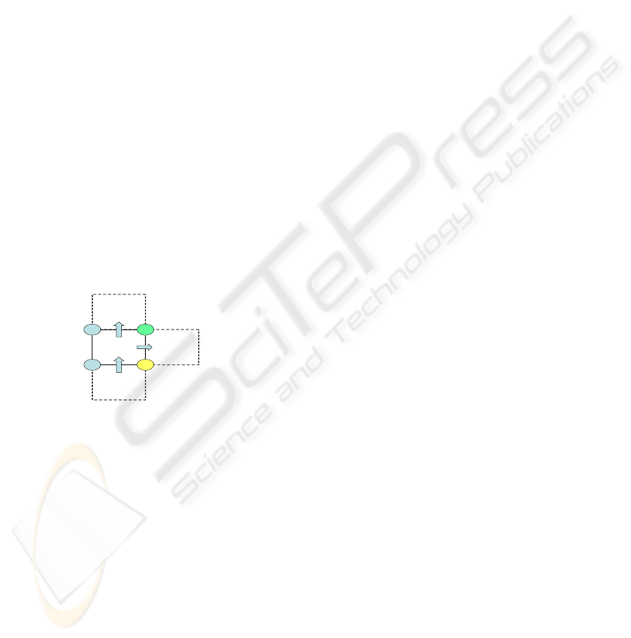
Figure 1: Next Cell Choices

The grid data structure holds status information

for each cell and the closest obstacle identification

for every corner of a grid cell. In a typical

implementation, both the cell status and the obstacle

identification can be stored in a single byte. Since

for a grid consisting of N x N cells there are (N+1)

corners, the number of bytes needed to store the

information associated with grid cells status and

corner information is given by: N

+ (N+1)

, which

is close to 2N

for large values of N, thus giving

O(N

). Therefore, for a 1000 x 1000 grid the

required amount of storage is around 2 Mbytes.

The proposed algorithm is based on three very

simple ideas. The first one is that all the vertices of

the working area bounding polygon are Voronoi

vertices. The second one derives from the

observation that the Voronoi diagram is always a

connected diagram, in which the Voronoi arcs

always have at least one intersection point. And the

third is that if at least 2 cell corners are closer to

different obstacles then the cell belongs to the

Voronoi Diagram. Therefore, given a starting point

for the diagram, it is possible to draw it on a grid by

checking at each step which is the next neighboring

cells to be visited. Such cells will be the ones whose

common edge with the current cell connects two

corners labeled with different obstacles and is not

the cell entrance edge. This procedure is shown

when a Voronoi vertex is reached on Figure 1.

Based on these three ideas the algorithm finds

the Voronoi diagram (VD) using the following

procedure:

begin

create a queue to temporarily hold the

Voronoi cells;

mark all the cells inside the working

area as free and all the cells

external and around the working area

as blocked;

choose one of the working area bounding

polygon vertices as the VD starting

point;

mark the corresponding cell as belonging

to the VD;

insert the starting point in the queue;

while the queue is not empty do

remove a cell from the queue;

mark it as belonging to the VD;

for each edge whose corner labels are

different

if it’s not the entrance edge and

not belonging to the diagram then

insert this neighbor cell in the

queue and fill in its corner's

label;

end if;

end for;

end while;

end;

The algorithm starts by choosing one of the

working area bounding polygon vertices as the

Voronoi diagram starting point and inserts it in the

temporary queue. Then, while this queue is not

empty, the algorithm removes cells from the queue

and marks them as belonging to the diagram. For

each cell marked, the next cell choice procedure is

used to determine which cells will be put in the

queue. All cells selected in the previous procedure

have their four corners labeled with the Euclidean

distance to the closest obstacle. Finally, the selected

cells are entered into the queue. The procedure is

repeated until no more cells can be found in the

queue. At this point the Voronoi diagram is

completely determined.

The amount of computation required for finding

the closest obstacle to a particular cell corner is

reduced if the algorithm computes only the distances

to obstacle edges which are “visible” from that

Possible

Position

Possible

Position

Last

Position

Present

Position

A B

ICINCO 2004 - ROBOTICS AND AUTOMATION

308

corner. A limited but effective visibility test of an

obstacle edge can be performed by finding the inner

product between a perpendicular outward vector to

the obstacle edge and a vector which starts at the cell

corner under consideration and points to any point

inside the obstacle polygon or on its edges. If the

inner product is negative, the edge is visible,

otherwise it is invisible and no distance calculations

need to be performed.

The procedure implemented by the described

algorithm would be sufficient to find the Voronoi

diagram for solving the path planning problem for

robots which are reduced to a point. In order to make

the algorithm work for arbitrarily shaped robots, a

slight modification has to be introduced. Let us

consider that the distance from the robot center to its

most external point is r. Then, when the algorithm

finds a cell which should belong to the Voronoi

diagram, it must perform a proximity test to verify if

the distances from all the cell corners to the closest

obstacles are greater than r. If this is true then the

cell is marked as belonging to the Voronoi diagram

and inserted in the queue. Otherwise the cell is

marked as blocked but it is still inserted in the

queue, because its neighbors may still belong to the

Voronoi diagram which will establish possible paths.

The algorithm error in defining the Voronoi

diagram is less than the size of a cell diagonal. If, for

instance, the robot working area is a 10m x 10m

square and the grid structure is defined as a 1000 x

1000 cell array, the maximum algorithm error is less

than 1.41 cm since the cell side is 1 cm long.

3 COOPERATIVE STRATEGY

The proposed cooperative implementation of the

algorithm described in Section 2 divides the working

area of the robots into Nr slices, where Nr is the

number of available robots. Each robot has a

working area slice associated with it and is

responsible for finding the Voronoi diagram within

that slice. Therefore, only a fraction (1/Nr) of the

grid data structure needs to be stored by each robot.

The data structure containing information on the

obstacle corner coordinates and on the equations of

the obstacle edges is broadcast to all the robots. Two

approaches have been adopted to solve this problem.

The first one does not require any communication,

but leads to some redundant work performed among

the robots. In the second approach, some

communication between the robots working on

neighbor slices is required but, as a consequence, a

more cooperative work pattern is adopted.

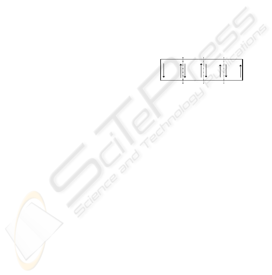
If we assume the working area is rectangular and

the cut lines are vertical lines, it is possible to say

that the Voronoi diagram will certainly cross the

vertical borders of a slice. So, in the first approach,

every robot searches both vertical border lines of its

assigned slice for grid cells representing Voronoi

points, as shown in Figure 2, where the use of four

processors (P0 to P3) is considered.

Once a Voronoi point is found, the Voronoi

diagram segment starting at the corresponding cell

and within robot slice is determined using the

algorithm described in Section 2. This procedure is

repeated until all the cells on both vertical border

lines have been visited. The two robots with the

leftmost and the rightmost slices assigned to them

can do less work because they know a priori the

working area corners are Voronoi vertices and,

therefore, they can draw the Voronoi diagram

segments starting from these two known points. So,

each vertical border line is analyzed twice by two

different robots as can be seen in Figure 2.

Figure 2: Working Area Partition

In the second approach, this redundant work is

avoided by assigning, for instance, the job of

searching a vertical border line to the robot which is

responsible for defining the Voronoi diagram within

the border right slice. The cell coordinates

corresponding to Voronoi points which have been

found on the border line are sent to the robot

processing the neighbor slice on the left. When the

coordinates of a cell are received, the robot puts the

cell on its queue. This cell will be used as the

starting point for finding a Voronoi diagram

segment. With this second approach, each robot

searches for Voronoi points on a single vertical

border line and receives the information on Voronoi

points on the other border line from its right side

neighbor. Therefore, each robot does less work and

uses communication to help its left side neighbor to

do its work.

4 EXPERIMENTAL RESULTS

The parallel algorithm described in Section 2 has

been implemented in C with the use of MPI

(Message Passing Interface) for implementing the

communication functions on an Ethernet cluster

consisting of 6 workstations, with 2.4 GHz Intel

Pentium 4 processors and 128 Mbytes of memory.

This environment has been chosen for the

experiments because it is similar to the actual

P1 P2

CONSTRUCTION OF THE VORONOI DIAGRAM BY A TEAM OF COOPERATIVE ROBOTS

309

environment in which the cooperative robots use

Ethernet-like wireless communication.

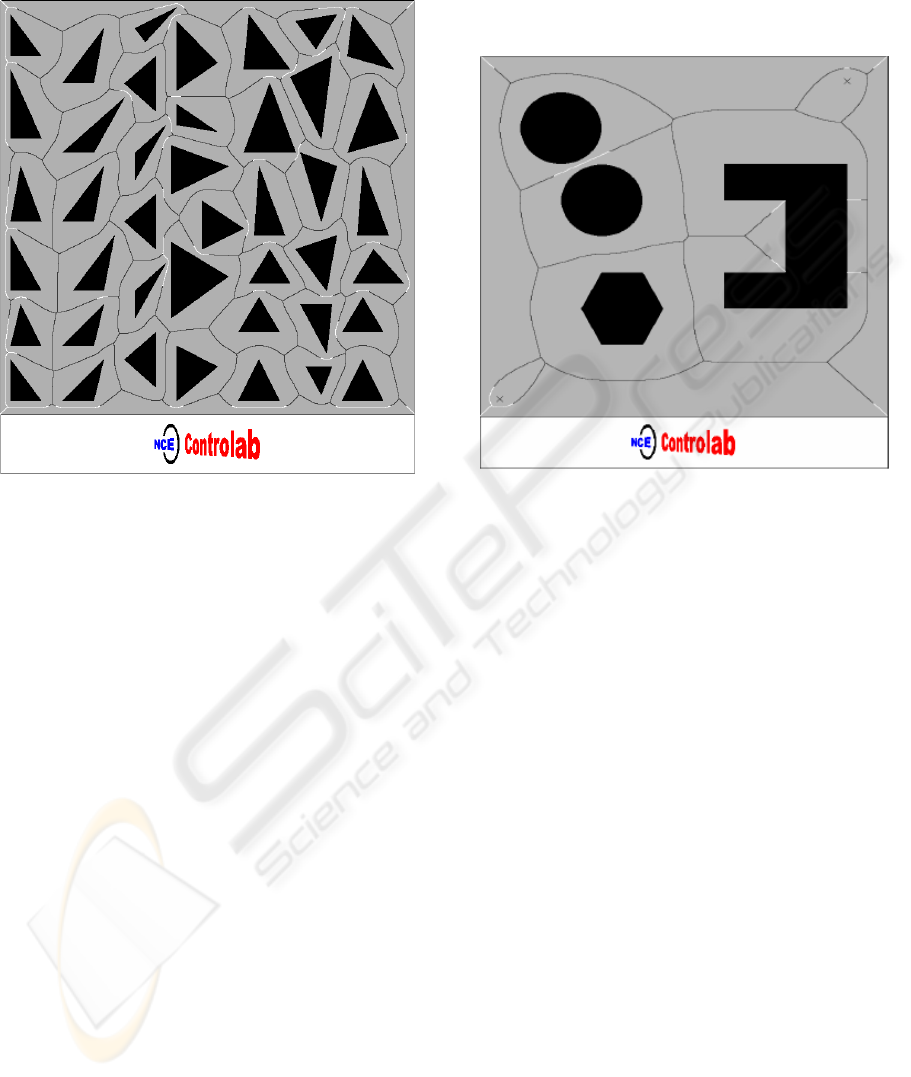
Figure 3: Voronoi Diagram – Sea of Triangles

Two obstacle arrangements have been

considered in the experimental work. In the first one,

a sea of triangles is placed within the working area.

Figure 3 shows the resulting Voronoi diagram

produced for this arrangement by the proposed

algorithm. The lighter lines represent Voronoi

diagram segments which have failed the proximity

test.

In the second example, less obstacles are present

but they have different types of shapes, including

circles, dots and non-convex polygons. Figure 4

shows the resulting Voronoi diagram for this

obstacle arrangement (mixed shapes).

For both obstacle arrangements shown in Figures

3 and 4, the application of the visibility test has been

able to reduce by nearly 40% the amount of

computational work performed by the algorithm.

For each example situation, three grid sizes have

been considered in the experiments: a small (1024 x

1024), a medium (2048 x 2048) and a large (4096 x

4096) one. For all combinations of obstacle

arrangements and grid sizes, both approaches for the

algorithm parallel implementation described in

Section 3 have been evaluated considering the use of

1, 2, 4 or 6 workstations in the network.

As a higher grid resolution is used, more work

has to be done by the processors in both approaches

(particularly in the no communication approach)

since the number of cells per slice border increases

and the number of Voronoi points in the diagram

also increases. However, the amount of work grows

linearly with the grid dimension. Therefore, the

algorithm performance can scale very well.

Figure 4: Voronoi Diagram - Mixed Shapes

It should also be noticed that the computational

work associated with the determination of Euclidean

distances between each candidate Voronoi point and

the visible edges is greater when the sea of triangles

arrangement is considered since the number of

obstacles is higher. This issue is important because,

with the no communication approach, the number of

Euclidean distances that are calculated is

approximately twice as big as the number of

distances evaluated by the cooperative approach. So,

when the amount of calculation is reduced, the no

communication approach was able to produce

smaller running times than the cooperative approach

in two situations in which only two processors were

in use, the grid size was not the largest one and the

mixed shape obstacle arrangement was considered.

Figures 5 and 6 show the speed up achieved by

the parallel algorithm based on both approaches.

The figures show that, in most cases, the

cooperative approach achieved a slightly higher

speed-up. Nevertheless, for both approaches the

speed up increases almost linearly with the number

of processors when the sea of triangles obstacle

arrangement is used. With this arrangement more

computational work is available to be done and, as a

consequence, better load balancing among a larger

number of processors can be achieved.

ICINCO 2004 - ROBOTICS AND AUTOMATION

310

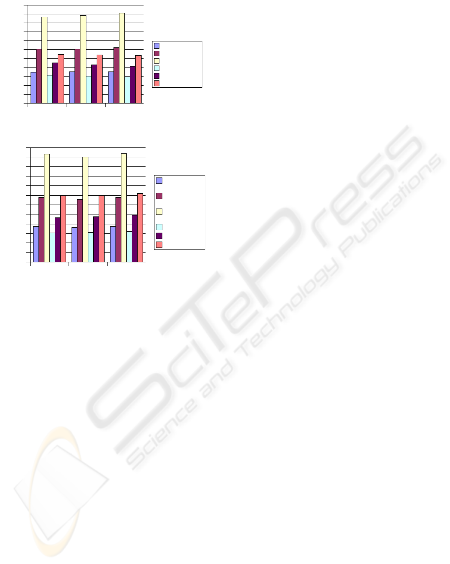
Figure 5: Speed-up - No Communication Approach

Figure 6: Speed-up - Cooperative Approach

5 CONCLUSIONS AND FUTURE

WORK

Two approaches for the cooperative implementation

of an algorithm for the construction of Voronoi

diagrams which is suitable for use within a team of

cooperative robots have been discussed in this paper.

The first one does not require any communication

among the robots. However, with this approach

some redundant work is performed by the robots.

The second approach requires some communication

among the robots but implements a more

cooperative strategy for the construction of the

Voronoi diagram.

Experiments performed on an Ethernet cluster of

workstations have demonstrated that both

approaches for the algorithm cooperative

implementation scale well with the number of

processors particularly when the number of

obstacles is big. Nevertheless, the approach based on

cooperation has produced slightly better results for

two quite different obstacle arrangements and for

different grid resolutions. With the achieved speed-

ups and running times, the parallel algorithm can be

used in applications where the obstacle

configuration changes with time within the robot

team working area and, consequently, real time path

re-planning is often needed.

Future work will include the actual

implementation and evaluation of the proposed

parallel algorithm within a team of cooperative

mobile robots under development in our laboratory

(Lopes, 2001) (Aude, 2003).

ACKNOWLEDGEMENTS

The authors would like to thank CNPq and FINEP

for the support given to the research work.

REFERENCES

E.P.L. Aude, et al., "CONTROLAB MUFA: A Multi-

Level Fusion Architecture for Intelligent Navigation

of a Telerobot", Proc. 1999 IEEE Int'l Conf. on

Robotics and Automation, Detroit, USA, May 1999,

V. 1, pp. 465-472

E.P.L. Aude, et al., “Real-Time Obstacle Avoidance

performed by an Autonomous Vehicle throughout a

Smoot Trajectory using an Electronic Stick”, Proc.

1999 IEEE Int'l Conf. on Robotics and Automation,

Las Vegas, USA, Oct 2003

J. Kim, P. Khosla, “Real-Time Obstacle Avoidance using

Harmonic Potential Functions”, Proc. of the IEEE Int'l

Conf. on Robotics and Automation, Sacramento, USA,

April, 1991, pp. 790-796

J.C. Latombe, “Robot Motion Planning”, Kluwer

Academic Publishers, USA, 1996

E.P. Lopes, et al., “Application of a Blind Person Strategy

for Obstacle Avoidance with the use of Potential

Fields”, Proc. 2001 IEEE Int'l Conf. on Robotics and

Automation, Seoul, Korea, May 2001

T. L. Pérez, W. R. Michael, “An Algorithm for Planning

Collision-Free Paths among Polyhedral Obstacles”,

Comm. of the ACM, V. 22, N. 10, Oct.1979, pp. 560-

570

N. Sudha, S. Nandi, K. Sridharan, “A Parallel Algorithm

to Construct Voronoi Diagram and its VLSI

Architecture”, Proc. of the 1999 IEEE Int'l Conf. on

Robotics and Automation, Detroit, USA, May , 1999,

pp. 1683-1688

P. G. Tzionas, , “Collision-Free Path Planning for a

Diamond-Shaped Robot Using Two-Dimensional

Cellular Automata”, IEEE Trans. on Robotics and

Automation, V. 13, N. 2, April 1997, pp. 237-250

1024 2048 4096

0,5

1,5

2,5

3,5

4,5

5,5

2 proc – tri-

angles

4 proc – tri-

angles

6 proc – tri-

angles

2 proc – mixed

4 proc – mixed

6 proc – mixed

Grid Size

Speed-Up

1024 2048 4096

0,5

1,5

2,5

3,5

4,5

5,5

2 proc – triangles

4 proc – triangles

6 proc – triangles

2 proc – mixed

4 proc – mixed

6 proc – mixed

Grid Size

Speed-Up

CONSTRUCTION OF THE VORONOI DIAGRAM BY A TEAM OF COOPERATIVE ROBOTS

311