EFFICIENT SYSTEM IDENTIFICATION FOR MODEL

PREDICTIVE CONTROL WITH THE ISIAC SOFTWARE

Paolino Tona

Institut Franc¸ais du P

etrole

1 & 4, avenue de Bois-Pr

eau, 92852 Rueil-Malmaison Cedex - France

Jean-Marc Bader

Axens

BP 50802 - 89, boulevard Franklin Roosevelt, 92508 Rueil-Malmaison Cedex - France

Keywords:

System identiﬁcation, model predictive control.

Abstract:

ISIAC (as Industrial System Identiﬁcation for Advanced Control) is a new software package geared to meet

the requirements of system identiﬁcation for model predictive control and the needs of practicing advanced

process control (APC) engineers. It has been designed to naturally lead the user through the different steps of

system identiﬁcation, from experiment planning to ready-to-use models. Each phase can be performed with

minimal user intervention and maximum speed, yet the user has every freedom to experiment with the many

options available. The underlying estimation approaches, based on high-order ARX estimation followed by

model reduction, and on subspace methods, have been selected for their capacity to treat the large dimensional

problems commonly found in system identiﬁcation for process control, and to produce fast and robust results.

Models describing parts of a larger system can be combined into a composite model describing the whole

system. This gives the user the ﬂexibility to handle complex model predictive control conﬁgurations, such as

schemes involving intermediate process variables.

1 INTRODUCTION

It is generally acknowledged that ﬁnding a dynamic

process model for control purposes is the most cum-

bersome and time-consuming step in model predic-

tive control (MPC) commissioning. This is mainly

due to special requirements of process industries that

make for difﬁcult experimental conditions, but also

to the relatively high level of expertise needed to ob-

tain empirical models through the techniques of sys-

tem identiﬁcation. The vast majority of MPC vendors

(and a few independent companies) have recognized

the need for efﬁcient system identiﬁcation and model

building tools and started providing software and fa-

cilities to ease this task.

In these pages, we present ISIAC (as Industrial

System Identiﬁcation for Advanced Control), a prod-

uct of the Institut Franc¸ais du P

etrole (IFP). This new

software package is geared to meet the requirements

of system identiﬁcation for model predictive control

and the needs of practicing advanced process control

(APC) engineers.

In section 2, we discuss the peculiarities of system

identiﬁcation for process control. Then we explain

how these peculiarities have been taken into account

in ISIAC design (section 3). Section 4 illustrates the

user workﬂow in ISIAC. Finally, section 5 presents

an example taken from an industrial MPC applica-

tion, carried out by Axens, process licensor ans ser-

vice provider for the reﬁning and petrochemical sec-

tors.

2 SYSTEM IDENTIFICATION

AND MODEL PREDICTIVE

CONTROL

With several thousands applications reported in the

literature, model predictive control (Richalet et al.,

1978; Cutler and Ramaker, 1980) technology has

been widely and successfully adopted in the process

industries, and more particularly, in the petrochemical

sector (see (Qin and Badgwell, 2003) for an overview

of modern MPC techniques).

The basic ingredients of any MPC algorithm are:

• a dynamic model, which is used to make an open-

loop prediction of process behavior over a chosen

future interval (the control model);

• an optimal control problem, which is solved at each

Tona P. and Bader J. (2004).

EFFICIENT SYSTEM IDENTIFICATION FOR MODEL PREDICTIVE CONTROL WITH THE ISIAC SOFTWARE.

In Proceedings of the First International Conference on Informatics in Control, Automation and Robotics, pages 86-93

DOI: 10.5220/0001142800860093

 SciTePress

control step, via constrained optimization, to min-

imize the difference between the predicted process

response and the desired trajectory;

• a receding horizon approach (only the ﬁrst step of

the optimal control sequence is applied).

Most commonly, control models employed by in-

dustrial MPC algorithms are linear time-invariant

(LTI) models, or, in same cases, combinations of LTI

models and static nonlinearities. The vast majority

of reported industrial applications have been obtained

utilizing ﬁnite impulse response (FIR) or ﬁnite step

response (FSR) models. Modern MPC packages are

more likely to use state-space, transfer function ma-

trix, or autoregressive with exogenous input (ARX)

models. Linear models of dynamic process behav-

ior can be obtained from a linearized ﬁrst-principles

model, or more commonly, from experimental mod-

eling, applying system identiﬁcation (Ljung, 1999)

techniques to obtain black-box models from input-

output data gathered from the process. Those mod-

els can be subsequently converted to the speciﬁc form

required by the MPC algorithm.

Several researchers have pointed out that process

identiﬁcation is the most challenging and demanding

part of a MPC project ((Richalet, 1993; Ogunnaike,

1996)). Although system identiﬁcation techniques

are basically domain independent, process industries

have special features and requirements that compli-

cate their use: slow dominant plant dynamics, large

scale units with many, strongly interacting, manipu-

lated inputs and controlled outputs, unmeasured dis-

turbances, stringent operating constraints. This makes

for difﬁcult experimental conditions, long test dura-

tions and barely informative data. But even the sub-

sequent step of performing system identiﬁcation us-

ing one of the available software packages may prove

lengthy and laborious, especially when the relatively

high level of expertise needed is not at hand.

Designing such software for efﬁciency and man-

ageability requires taking into account the peculiari-

ties of system identiﬁcation for process control.

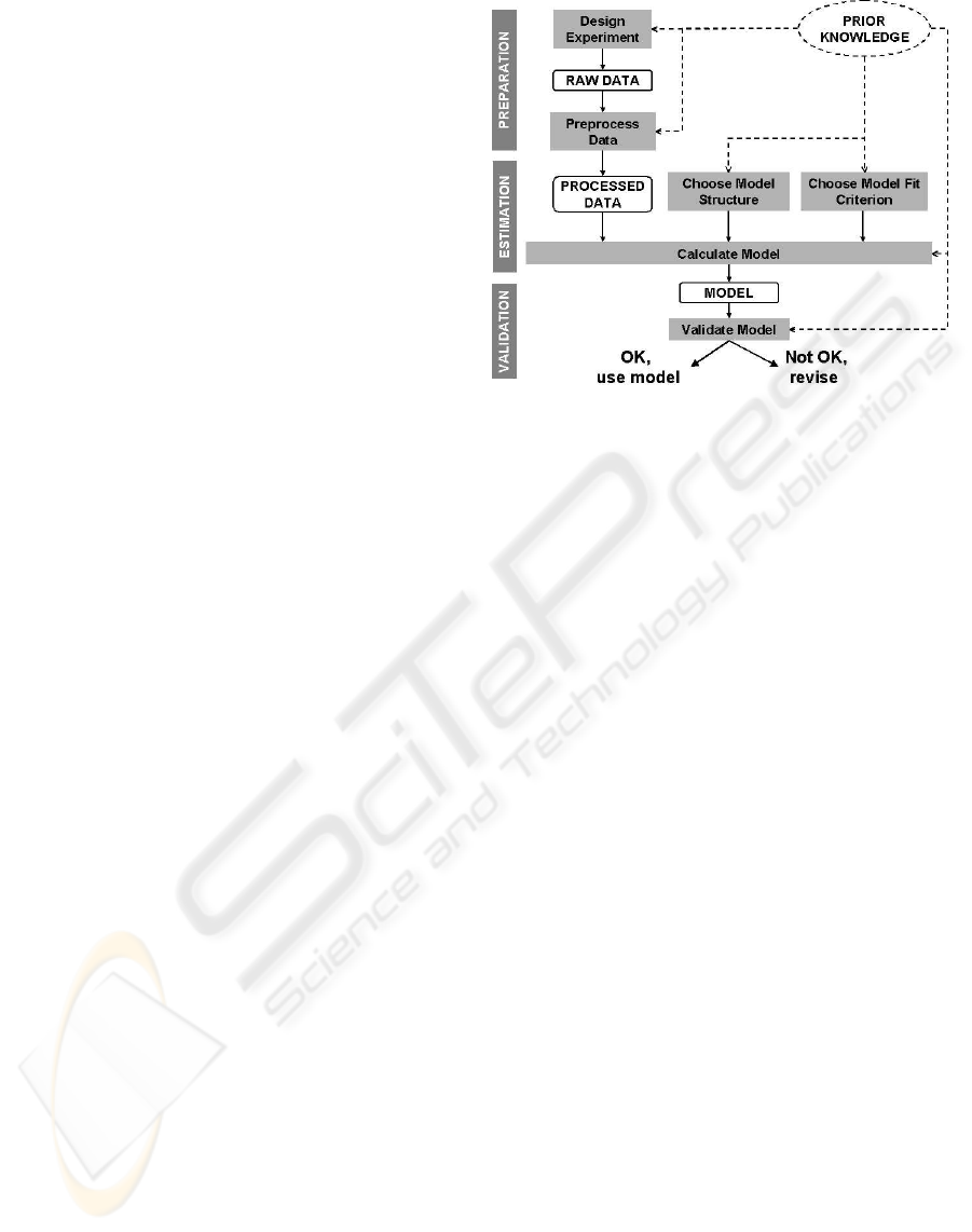
• System identiﬁcation is a complex process involv-

ing several steps (see Fig. 1). The user should be

guided through it with a correct balance between

structure and suppleness.

• When identifying an industrial process, a signiﬁ-

cant number of data records must be dealt with.

Data may contain thousands of samples of tens

(or hundreds) measured variables. Several differ-

ent multivariable models can be identiﬁed for the

whole process, or for parts of it. It is important to

allow the user to handle multiple models and data

sets of any size, to seamlessly visualize, evaluate,

compare and combine them, to arrange and keep

track of the work done during an identiﬁcation ses-

sion.

Figure 1: Steps of the system identiﬁcation process

(adapted from (Ljung, 1999))

• Estimation and validation methods at the heart of

the identiﬁcation process must be chosen care-

fully. When dealing with multi-input multi-

output (MIMO) models, model structure choice

and parametrization may prove challenging even

for experienced users. Moreover, large data and

model sizes, utterly common in the context of sys-

tem identiﬁcation for process control, may eas-

ily lead to numerical difﬁculties and unacceptable

computation times. Methodologies giving system-

atic answers to these problems exist (Juricek et al.,

1998; Zhu, 1998) and have been incorporated into

some commercial packages (Larimore, 2000; Zhu,

2000).

• MPC algorithms usually need more information to

deﬁne their internal control structure, than a plain

linear model. As a minimum, the user has to sort

model inputs into manipulated variables (MV) and

disturbance variables (DV), and to choose which

model outputs are to be kept as controlled vari-

ables (CV). With modern MPC packages, control

conﬁguration may become really complex, includ-

ing observers and unmeasured disturbance models,

which can be used, among other things, to take into

account the presence of intermediate variables (i.

e., measured output variables that inﬂuence con-

trolled variables) for control calculation. Without

a suitable control model building tool, supplying

the additional pieces of information turns out to be

a laborious task, even for mildly complex control

conﬁgurations.

EFFICIENT SYSTEM IDENTIFICATION FOR MODEL PREDICTIVE CONTROL WITH THE ISIAC SOFTWARE

3 ISIAC

ISIAC is primarily meant to support the model-based

predictive multivariable controller MVAC, a part of

the APC suite developed by IFP and its afﬁliate RSI.

MVAC has ﬁrst been validated on a challenging

pilot process unit licensed by IFP (Couenne et al.,

2001), and is currently under application in several

reﬁneries world-wide. Its main features are:

• state-space formulation;

• observer to take into account unmeasured distur-

bances, intermediate variables, integrating behav-

ior;

• ranked soft and hard constraints;

• advanced speciﬁcation of trajectories (funnels, set-

ranges);

• static optimization of process variables.

Though ISIAC is intended to be the natural com-

panion tool to MVAC, it is actually ﬂexible enough

to be used as a full-ﬂedged system identiﬁcation and

model building tool or to support other APC pack-

ages.

3.1 Approaches to model estimation

The model estimation approaches selected for inclu-

sion in ISIAC combine accuracy and feasibility, both

in term of computational requirements and of user

choices. We have decided to favor non-iterative meth-

ods over prediction error methods (Ljung, 1999),

to avoid problems originating from a demanding

minimization routine and a complicated underlying

parametrization.

3.1.1 Two-stage method

The beneﬁts of high-order ARX estimation in indus-

trial situations have been advocated by several re-

searchers ((Zhu, 2001; Rivera and Jun, 2000)). In-

deed, using a model order high enough, and with

sufﬁciently informative data, ARX estimation yields

models that can approximate any linear system arbi-

trarily well (Ljung, 1999). Ljung’s asymptotic black-

box theory also provides (asymptotic) expressions for

the transfer function covariance which can be used for

model validation purposes.

A model reduction step is necessary to use these

models as process control models, since they usually

are over-parameterized (i.e., an unbiased model with

much lower order can be found) and have high vari-

ance (which is roughly proportional to model order).

Different schemes have been proposed ((Hsia, 1977;

Wahlberg, 1989; Zhu, 1998; Rivera and Jun, 2000;

arnstr

om and Ljung, 2003)) to perform model re-

duction. For a class of reduction schemes (Tj

arnstr

and Ljung, 2003), it has been demonstrated that the

reduction step actually implies variance reduction,

and a resulting variance which is nearly optimal (that

is, close to the Cramer-Rao bound).

In ISIAC, truly multi-input multi-output (MIMO)

ARX estimation is possible, using the structure

A(q)y(t) = B(q)u(t) + e(t)

where y(t) is the p-dimensional vector of outputs

at time t, u(t) is the m-dimensional vector of in-

puts at time t, e(t) is a p-dimensional white noise

vector, A(q) and B(q) polynomial matrices respec-

tively of dimensions p × p and p × m. For faster

results, in the two-stage method, the least-square es-

timation problem is decomposed into p multi-input

single-output (MISO) problems. The Akaike infor-

mation criterion (AIC) (Ljung, 1999) is used to ﬁnd

a “high enough” order in the ﬁrst step, and the re-

sulting model is tested for unbiasedness (whiteness

of the residuals and of the inputs-residuals cross-

correlation). To ﬁnd a reduced order model, we adopt

a frequency-weighted balanced truncation (FWBT)

technique (Varga, 1991). The calculated asymptotic

variance is used to set the weights and to automat-

ically choose the order of the reduced model, fol-

lowing an approach inspired by (Wahlberg, 1989).

The obtained model is already in the state-space form

needed by the MPC algorithm.

As a result, we get an estimation method which

is totally automated, and provides accurate results in

most practical situations, with both open-loop and

closed-loop data. Yet, this method might not work

correctly when dealing with short data sets and (very)

ill-conditioned systems.

3.1.2 Automated subspace estimation

The term subspace identiﬁcation methods (SIM)

refers to a class of algorithms whose main charac-

teristic is the approximation of subspaces generated

by the rows or columns of some block matrices of

the input/output data (see (Bauer, 2003) for a recent

overview). The underlying model structure is a state-

space representation with white noise (innovations)

entering the state equation through a Kalman ﬁlter

and the output equation directly

x(t + 1) = Ax(t) + Bu(t) + Ke(t)

y(t) = Cx(t) + Du(t) + e(t)

Simplifying (more than) a bit a fairly complex theory,

input and output data are used to build an extended

state-space system, where both data and model infor-

mation are represented as matrices, and not just vec-

tor and matrices. Kalman ﬁlter state sequences are

then identiﬁed and used to estimate system matrices

A, C, and, if a disturbance model is needed, K (B and

D can be subsequently estimated in several different

ICINCO 2004 - SIGNAL PROCESSING, SYSTEMS MODELING AND CONTROL

ways). This can be assimilated (Ljung, 2003) to the

estimation of a high-order ARX model, which is then

reduced using weighted Hankel-norm model reduc-

tion. The three most well-known algorithms, CVA,

N4SID and MOESP, can be studied under an uni-

ﬁed framework (Van Overschee and DeMoor, 1996),

where each algorithm stems from a different choice

of weightings in the model reduction part. Subspace

identiﬁcation methods can handle the large dimen-

sional problems commonly found in system identiﬁ-

cation for process control, producing (very) fast and

robust results. However, it must be pointed out that

their estimates are generally less accurate than those

from prediction error methods and that standard SIM

algorithms are biased under closed-loop conditions.

Even though a lower accuracy is to be expected, it

is important to have a viable alternative to the two-

step method. This is why, we have implemented in

ISIAC two estimation procedures based on subspace

algorithms taken from control and systems library

SLICOT (Benner et al., 1999):

• a combined method, where MOESP is used to es-

timate A and C and N4SID is used to estimate B

and D;

• a simulation method, where MOESP is used to es-

timate A and C and linear regression is used to es-

timate B and D.

The second method is usually more accurate (though

a little slower) and is presented as the default choice.

High-level design parameters for these two method-

ologies are the ﬁnal model order n, and the prediction

horizon r used in the model reduction step. ISIAC

can select both parameters automatically: the latter

using a modiﬁed AIC criterion based on a high-order

ARX estimation, the former using a combined crite-

rion taking into account the relative importance of sin-

gular values and errors on simulated outputs (output

errors).

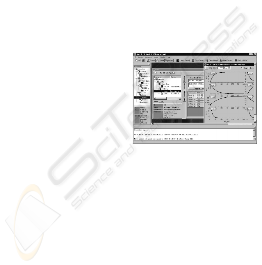
3.2 General structure and layout

Fig. 2 shows ISIAC graphical user interface (GUI).

The tree on the left (the session tree) highlights the

relationships between the different elements the user

deals with during a typical system identiﬁcation ses-

sion.

• A System object representing the whole process the

user is working on. It includes a list of process

Variables and a list of Subsystems, which can be

used to store partial measurements and dynamic

models relating groups of input and output vari-

ables.

• Data objects in two ﬂavors: Raw Data and IO

Data. The former are deﬁned from raw process

data records and do not carry any structure infor-

mation. They are mainly used for preliminary ap-

praisal and processing of available data sets. IO

data are deﬁned by selecting subsets of ﬁelds of raw

data objects, and can be used for system identiﬁca-

tion. Notice that data objects in ISIAC may include

measurements coming from different experiments

(multi-batch data).

• Models include all the dynamic models estimated

or deﬁned during a session. ISIAC handles

discrete-time state-space, transfer function (ma-

trix), FIR, ARX and general polynomial models.

State-space and transfer function models are also

available in continuous time. Simple process mod-

els, such as ﬁrst-order plus time delay (FOPTD)

models in gain-time constant-delay form, are han-

dled as specializations of transfer function models.

Figure 2: ISIAC GUI

This structure provide a powerful and ﬂexible sup-

port to the user:

• no restriction is put on the number of models and

data objects, nor on their sizes;

• system identiﬁcation of the whole process can be

decomposed in smaller problems whose results can

be later recombined;

• it is straightforward to keep track of all the work

done during an identiﬁcation session.

Three special windows are dedicated to deﬁnition

and basic handling of system, data and model objects.

The Input Design Window is intended to help the user

to design appropriate test signals for system identiﬁ-

cation. More advanced operations on data and mod-

els are available in the Data Processing Window and

in the Model Processing Window. The most impor-

tant window is certainly the Data To Models Window,

where model estimation and validation take place.

Last, the ISIAC To MVAC Window hosts the graphi-

cal control model builder.

EFFICIENT SYSTEM IDENTIFICATION FOR MODEL PREDICTIVE CONTROL WITH THE ISIAC SOFTWARE

ISIAC GUI implements a multi-document inter-

face (MDI) approach: it is possible to have several

windows opened at once in the child window area.

Furthermore, thanks to drag-and-drop operations and

pop-up menus, the same action (say, plotting a model

time response) is accessible from different locations.

This means that, although ISIAC layout clearly under-

lines the different steps of the identiﬁcation process,

the user is never stuck into a ﬁxed workﬂow.

4 WORKING WITH ISIAC

4.1 Experiment design

Whenever the APC engineer has the freedom to

choose other input moves than classical step-testing

(not often, unfortunately), ISIAC offers support to

generate test signals which are more likely to yield

informative data. The Input Design Window lets the

user design signals such as pseudo-random binary sig-

nals (PRBS), using few high level parameters.

4.2 Working with data

As mentioned before, ISIAC data objects provide a

structure to handle measurements of process vari-

ables. Input ﬁles containing raw measurements do

not need to carry any special information (other than

including delimited columns of values), and can be

imported without any external spreadsheet macro,

since data object formatting is done interactively into

ISIAC Data Window. Data visualization tools, which

include stacked plots, single-axis plots and various

statistical plots, have been designed with particular

care.

The more advanced functions of the Data Process-

ing Window are those commonly found in industrial

system identiﬁcation packages: normalization, de-

trending, de-noising, re-sampling, ﬁltering, nonlinear

transformations, data slicing, data merging. Notice

that a set of these data processing operations is incor-

porated in the automated model identiﬁcation proce-

dure (see section 4.4).

4.3 Working with models

Most commonly, dynamic process models in ISIAC

are estimated from data or obtained combining or

processing existing (estimated) models. Models can

be also directly deﬁned by the user (in FOPTD

form, for instance) or imported from other packages.

ISIAC Model Window also provides transformations

between different LTI representations and time do-

main conversions, as well as several analysis and vi-

sualization tools. Model response plots, both in time

domain and in frequency domain, are extremely ﬂex-

ible. An unlimited number of models (not necessarily

sharing the same inputs or outputs) can be compared

on the same chart, and an unlimited number of chart-

ing windows can be opened at once.

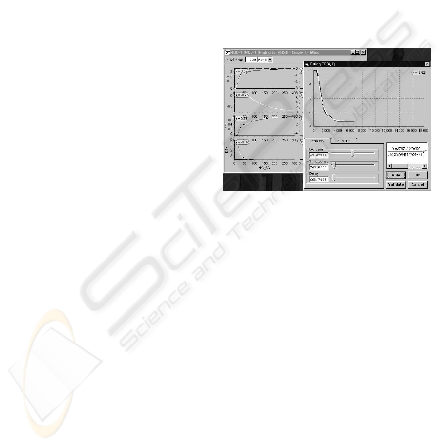
Advanced model processing (in the Model Pro-

cessing Window) includes model reduction and model

building tools. Time domain techniques (step re-

sponse ﬁtting of simple process models, see Fig. 3) or

frequency weighted model reduction techniques are

available. Model building can be performed through

simple connections (cascade, parallel) or through a

full-ﬂedged graphical model builder which closely re-

sembles the one described in section 4.5.

Figure 3: Step response ﬁtting

4.4 Estimating and validating

models

Model estimation must be preceded by some amount

of data processing, namely offset removal, normal-

ization and detrending (that is, removal of drifts and

low frequency disturbances). In ISIAC, these basic

but essential transformation are automatically applied

(unless the user does not want to), in a transparent

manner, before model estimation. Actually the Data

Processing Window, is only necessary when more ad-

vanced data processing is needed. Moreover, prior in-

formation about certain characteristics of the system

(integrating behavior, input-output delay) can be also

incorporated to help the estimation algorithms.

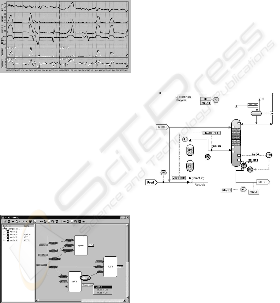
As explained in section 3.1, the default estima-

tion method in ISIAC is the two-stage method. This

method, combined with the transparent basic data

processing, results in a “click&go” approach that is

greatly appreciated by industrial practitioners. The in-

dustrial example of Fig. 4 shows that with this method

the user can really make the most of the available data,

even when the inputs are not very informative. Alter-

natively, subspace estimation can be selected. It is

ICINCO 2004 - SIGNAL PROCESSING, SYSTEMS MODELING AND CONTROL

also possible to estimate FIR models or general ARX

models.

Beside the comparison between measured outputs

and simulated outputs (as in Fig. 4), model validation

can be performed by checking the conﬁdence bounds

and visualizing and comparing time and frequency re-

sponses.

Figure 4: Model validation through simulation (simulated

outputs in white)

4.5 Building the control model

One of the most interesting features of ISIAC is

the graphical control model builder, in the ISIAC To

MVAC Window (Fig. 5). With a few mouse clicks,

it is possible to build a complex control model from

a combination of sub-models, identiﬁed from differ-

ent data sets or extracted from existing models. The

user is only required to indicate the role of each input

and output in the control scheme. The model graph

can be then translated into a control model with the

appropriate format, or into a plant model for off-line

simulations. The resulting plant model can be also

transferred back to ISIAC workspace and applied to

the existing data sets to verify its correctness.

Figure 5: The graphical control model builder

The model builder proves particularly helpful when

intermediate process variables are to be included. In

ﬁgure 5, which depicts part of the control conﬁgura-

tion for a unit involving cascaded reactors, the vari-

able denoted S HDT 1 is one of those variables.

5 AN INDUSTRIAL

APPLICATION: MODEL

PREDICTIVE CONTROL OF A

MTBE UNIT

To prove the usefulness of ISIAC in an industrial con-

text, we examine some aspects of a model predictive

control project, carried out by IFP afﬁliate Axens on

a petrochemical process unit.

The process under consideration is an etheriﬁca-

tion unit producing methyl-tert-butyl ether (MTBE),

from a reaction between isobutene (IB) and methanol

(MeOH).

Figure 6: The MTBE unit

The key control objectives are:

• maximize MTBE yield;

• increase IB recovery;

• reduce steam consumption;

• control MTBE purity.

The MVAC-based control system includes 7 MVs,

3 DVs, 6 CVs, with 5 intermediate variables. In the

following, we only consider a subset corresponding

to the control of MeOH percentage in MTBE (last

item of the objective list). Fig. 7 shows, from a sys-

tem viewpoint, how the controlled variable MEOH

IN MTBE is inﬂuenced by others process variables

of the control conﬁguration:

• feed ﬂow, MeOH ﬂow and sensitive temperature of

the catalytic column as CVs;

EFFICIENT SYSTEM IDENTIFICATION FOR MODEL PREDICTIVE CONTROL WITH THE ISIAC SOFTWARE

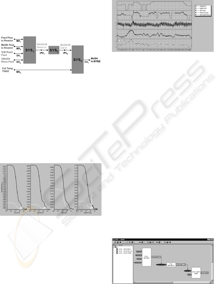
• IB and MeOH percentages in feed to ﬁrst reactor as

DVs;

• the ratios of MeOH over IB, respectively entering

the ﬁrst reactor and the catalytic column, as inter-

mediate variables.

Figure 7: Part of the MTBE control scheme

There are several avantages in introducing interme-

diate variables in the control conﬁguration, instead of

considering only direct transfer functions between in-

put variables (MVs plus DVs) and the CV:

• intermediate variables can be bounded, for tighter

control;

• unavoidable uncertainties in cascaded models (up-

stream from intermediate variables) can be com-

pensated for;

• deviations from predicted behavior can be detected

long before they affect the CV.

Figure 8: Frequency response of an identiﬁed model for

subsystem SYS1

ISIAC has been used for data visualization and

analysis, as well as for identiﬁcation of sub-models

later included in the overall control conﬁguration. As

an example, we present some identiﬁcation results re-

lating to subsystem SYS1 of Fig. 7. Fig. 8 shows

the frequency response of a high order ARX model

together with its error bounds. The estimates of the

ﬁrst two transfer functions (MV

→ iP V

, MV

→

iP V

) appear to be fairly accurate, since their error

bounds are comparatively quite small. The overall

quality of estimation is conﬁrmed by the comparison

between measured and predicted output (ﬁgure 9).

Figure 9: Measured vs. predicted (white) output for subsys-

tem SYS1

As for control model building, Fig. 10 shows how

naturally the dedicated graphical tool translates block

diagrams like the one in Fig. 7. From this graphical

representation, it takes only one mouse-click to gen-

erate scripts for simulation purposes or for ﬁnal MPC

implementation.

6 CONCLUSION

ISIAC proposes a modern, ﬂexible and efﬁcient

framework to perform system identiﬁcation for ad-

vanced process control. Its main strengths are:

• a graphical user interface which emphasizes the

multi-step nature of the identiﬁcation process,

without trapping the user into a ﬁxed workﬂow;

• fast and robust estimation methods requiring mini-

mal user intervention;

• no restriction on the number or on the size of data

sets and models the user can work with;

• full support for the speciﬁcation of complex model

predictive control schemes, by means of block dia-

gram combination of (linear) models.

Through an exemple taken from an industrial MPC

application, we have illustrated the advantages of us-

ing our software in a concrete situation.

Figure 10: Building the partial MTBE control scheme in

ISIAC

ICINCO 2004 - SIGNAL PROCESSING, SYSTEMS MODELING AND CONTROL

REFERENCES

Bauer, D. (2003). Subspace algorithms. In Proc. of the 13th

IFAC Symposium on System Identiﬁcation, Rotterdam,

NL.

Benner, P., Mehrmann, V., Sima, V., Van Huffel, S., and

Varga, A. (1999). SLICOT, a subroutine library in sys-

tems and control theory. Applied and Computational

Control, Signals and Circuits, 1:499–539.

Couenne, N., Humeau, D., Bornard, G., and Chebassier,

J. (2001). Contr

ole multivariable d’une unit

e de

eparation des xyl

enes par lit mobile simul

e. Revue

de l’Electricit

e et de l’Electronique, 7-8.

Cutler, C. R. and Ramaker, B. L. (1980). Dynamic matrix

control: a computer control algorithm. In Proc. of

the American Control Conference, San Francisco, CA,

USA.

Hsia, T. C. (1977). Identiﬁcation: Least Square Methods.

Lexington Books, Lexington, Mass., USA.

Juricek, B. C., Larimore, W. E., and Seborg, D. E. (1998).

Reduced-rank ARX and subspace system identiﬁca-

tion for process control. In Proc. IFAC DYCOPS Sym-

pos., Corfu, Greece.

Larimore, W. (2000). The ADAPTx software for automated

multivariable system identiﬁcation. In Proc. of the

12th IFAC Symposium on System Identiﬁcation, Santa

Barbara, CA, USA.

Ljung, L. (1999). System Identiﬁcation, Theory for the

User. Prentice-Hall, Englewood Cliffs, NJ, USA, sec-

ond edition.

Ljung, L. (2003). Aspects and experiences of user choices

in subspace identiﬁcation methods. In Proc. of the

13th IFAC Symposium on System Identiﬁcation, Rot-

terdam, NL.

Ogunnaike, B. A. (1996). A contemporary industrial per-

spective on process control theory and practice. A.

Rev. Control, 20:1–8.

Qin, S. J. and Badgwell, T. A. (2003). A survey of indus-

trial model predictive control technology. Control En-

gineering Practice, 11:733–764.

Richalet, J. (1993). Industrial applications of model based

predictive control. Automatica, 29(5):1251–1274.

Richalet, J., Rault, A., Testud, J. L., and Papon, J. (1978).

Model predictive heuristic control: applications to in-

dustrial systems. Automatica, 14:414–428.

Rivera, D. E. and Jun, K. S. (2000). An integrated identiﬁca-

tion and control design methodology for multivariable

process system applications. IEEE Control Systems

Magazine, 20:2537.

arnstr

om, F. and Ljung, L. (2003). Variance properties

of a two-step ARX estimation procedure. European

Journal of Control, 9:400 –408.

Van Overschee, P. and DeMoor, B. (1996). Subspace Iden-

tiﬁcation of Linear Systems: Theory, Implementation,

Applications. Kluwer Academic Publishers.

Varga, A. (1991). Balancing-free square-root algorithm for

computing singular perturbation approximations. In

Proc. of 30th IEEE CDC, Brighton, UK.

Wahlberg, B. (1989). Model reduction of high-order esti-

mated models: The asymptotic ML approach. Inter-

national Journal of Control, 49:169–192.

Zhu, Y. (1998). Multivariable process identiﬁcation for

MPC: the asymptotic method and its applications.

Journal of Process Control, 8(2):101–115.

Zhu, Y. (2000). Tai-Ji ID: Automatic closed-loop identiﬁca-

tion package for model based process control. In Proc.

of the 12th IFAC Symposium on System Identiﬁcation,

Santa Barbara, CA, USA.

Zhu, Y. (2001). Multivariable System Identiﬁcation for Pro-

cess Control. Elsevier Science Ltd.

EFFICIENT SYSTEM IDENTIFICATION FOR MODEL PREDICTIVE CONTROL WITH THE ISIAC SOFTWARE