POLYNOMIAL ESTIMATION OF SIGNALS FROM UNCERTAIN
OBSERVATIONS USING COVARIANCE INFORMATION
S. Nakamori
Department of Technology. Faculty of Education, Kagoshima University
1-20-6, Kohrimoto, Kagoshima 890-0065, Japan
R. Caballero-
´
Aguila
Departamento de Estad
´
ıstica e Investigaci
´
on Operativa, Universidad de Ja
´
en
Paraje Las Lagunillas, s/n, 23071 Ja
´
en, Spain
A. Hermoso-Carazo and J. Linares-P
´
erez
Departamento de Estad
´
ıstica e Investigaci
´
on Operativa, Universidad de Granada
Campus Fuentenueva, s/n, 18071 Granada, Spain
Keywords:
Uncertain observations, polynomial estimation, covariance information.
Abstract:
The least-squares ν th-order polynomial filtering and fixed-point smoothing problems of uncertainly observed
signals are considered. The proposed estimators do not require the knowledge of the state-space model gener-
ating the signal, but only the moments (up to the 2νth one) of the signal and the observation noise, as well as
the probability that the signal exists in the observations.
1 INTRODUCTION
Systems with uncertain observations are character-
ized by including an observation multiplicative noise
described by a sequence of Bernoulli random vari-
ables whose values -one or zero- indicate the pres-
ence or absence of signal in the observation, respec-
tively. So, these systems constitute an appropriate
model for analyzing those situations in which the ob-
servation may not contain the signal to be estimated
and, hence, it consists only of noise (for example, sit-
uations of fading or reflection of transmitted signals
from the ionosphere).
Due to the multiplicative noise component, even if
the additive observation noise is gaussian, the least-
squares (LS) estimator is not a linear function of the
observations and, usually, it is not easily obtainable.
This difficulty has motivated the necessity of looking
for suboptimal estimators which are easier to obtain;
particularly, linear and polynomial estimation prob-
lems from uncertain observations have been treated
by several authors, as NaNacara and Yaz (1997), Ca-
ballero et al. (2003), etc., assuming a full knowledge
of the state-space model for the signal process.
Nevertheless, usually the state-space model is not
available and the estimation problem must be ad-
dressed using another kind of information, such as
covariance information about the processes involved.
The LS linear estimation problem from uncertain ob-
servations using this kind of information has been
considered, for example, in Nakamori et al. (2003a)
and these results are extended in Nakamori et al.
(2003b) by proposing algorithms for the LS quadratic
estimators, which improve the linear ones.
In this paper the results in Nakamori et al. (2003a,
2003b) are generalized. More specifically, we address
the LS polynomial filtering and fixed-point smooth-
ing problems of arbitrary degree (ν) from uncertain
observations perturbed by white noise. Besides the
probability that the signal exists in the observations,
the proposed estimators only require the knowledge
of the moments (up to the 2νth one) of the signal and
the observation additive noise.
2 PROBLEM FORMULATION
Let z(k) and y(k) be n × 1 vectors describing the
signal and its observation at time k, respectively. Let
us suppose that
y(k) = U(k)z(k) + v(k). (1)
Our aim is to obtain the least-squares (LS) νth-
order polynomial estimator of the signal z(k) based
305
Nakamori S., Caballero-Águila R., Hermoso-Carazo A. and Linares-Pérez J. (2004).
POLYNOMIAL ESTIMATION OF SIGNALS FROM UNCERTAIN OBSERVATIONS USING COVARIANCE INFORMATION.
In Proceedings of the First International Conference on Informatics in Control, Automation and Robotics, pages 307-311
DOI: 10.5220/0001126903070311
Copyright
c
 SciTePress

on the observations {y(1), . . . , y(L)}, being ν ≥ 1
arbitrary. Defining the random vectors
y
[2]
(i) = y(i) ⊗ y(i)
y
[j]
(i) = y
[j−1]
(i) ⊗ y(i), j > 2
(⊗ denotes the Kronecker product, Magnus and
Neudecker (1988)), and assuming that E
£
y
[2ν]
(i)
¤
<
∞, this estimator is the orthogonal projection of
z(k) on the space of n-dimensional linear transforma-
tions of y(1), . . . , y(L) and their Kronecker powers
y
[2]
(1), . . . , y
[ν]
(1), . . . , y
[2]
(L), . . . y
[ν]
(L). More
specifically, we are interested in obtaining the LS
νth-order polynomial filter (L = k) and fixed-point
smoother (L > k) of the signal. For this purpose, we
assume the following hypotheses:
(H.1) The signal process {z(k); k ≥ 0} has zero
mean and, for i, j = 1, . . . , ν, the covariance func-
tion of the vectors z
[i]
(k) and z
[j]
(k), K
ij
(k, s) =
E[z
[i]
(k)z
[j]
T
(s)], can be expressed as
K
ij
(k, s) =
½
A
ij
(k)B
T
ij
(s), 0 ≤ s ≤ k
B
ji
(k)A
T
ji
(s), 0 ≤ k ≤ s
where A
ij
and B
ij
are n
i
× N
ij
and n
j
× N
ij
known
matrix functions, respectively, and
x := x − E[x].
(H.2) The noise process {v(k); k ≥ 0} is a zero-
mean white sequence with E[v
[2ν]
(k)] < ∞ and
E[v
[i]
(k)] is known for i = 1, . . . , 2ν.
(H.3) The multiplicative noise {U(k); k ≥ 0} is a
sequence of independent Bernoulli random variables
with known P [U(k) = 1] = p(k).
(H.4) The processes {z(k); k ≥ 0}, {U (k); k ≥ 0}
and {v(k); k ≥ 0} are mutually independent.
To address the LS νth-order polynomial estimation
problem, we define the augmented signal and obser-
vation vectors as
Z(k) =



z(k)
.
.
.
z
[ν]
(k)



, Y(k) =



y(k)
.
.
.
y
[ν]
(k)



.
Then, the vector constituted by the first n en-
tries of the LS linear estimator of Z(k) based on
Y(1), . . . , Y(L) provides the LS νth-order polyno-
mial estimator of the original signal z(k).
Next we study the properties of Z(k) and Y(k)
which will be used to obtain the LS linear estimator
of Z(k).
3 AUGMENTED EQUATION
In order to analyze the properties of the vector Y(k),
we start by obtaining an appropriate expression for
y
[j]
(k), j = 2, . . . , ν. By employing the Kronecker
product properties and noting that U(k) = U
2
(k) =
· · · = U
ν
(k), y
[j]
(k) can be written as
y
[j]
(k) = U(k)
j
X
l=1
L
jl
(k)z
[l]
(k)+E[v
[j]
(k)]+g
j
(k).
where
L
jl
(k) = M
j
j−l
(n)
¡
E[v
[j−l]
(k)] ⊗ I
n,l
¢
, l ≤ j − 1
L
jj
(k) = I
n,j
and
g
j
(k) = U(k)
j−1
X
l=1
M
j
j−l
(n)
³
v
[j−l]
(k) ⊗ I
n,l
´
z
[l]
(k)
+
v
[j]
(k)
with
M
j
0
(n) = M
j
j
(n) = I
n,j
,
M
j
r
(n) = (M
j−1
r
(n) ⊗ I
n,1
)
+(M
j−1
r−1
(n) ⊗ G
j−r
), 1 ≤ r ≤ j − 1
G
l
= (I
n,1
⊗ G
l−1
)(G
1
⊗ I
n,l−1
), G
1
= K
n,n
(I
n,l
denotes the n
l
×n
l
identity matrix; K
n,m
is the
nm × nm commutation matrix).
Then, by denoting
C(k) =



L
11
(k) 0
n×n
2
· · · 0
n×n
ν
L
21
(k) L
22
(k) · · · 0
n
2
×n
ν
· · · · · · · · · · · ·
L
ν1
(k) L
ν2
(k) · · · L
νν
(k)



,
V
k
=





0
n×1
E{v
[2]
(k)}
.
.
.
E{v
[ν]
(k)}





, G(k) =




v(k)
g
2
(k)
.
.
.
g
ν
(k)




we obtain that Y (k) = Y(k) − E[Y(k)] satisfy the
following augmented observation equation
Y (k) = U(k)C(k)Z(k) + V (k) (2)
where Z(k) = Z(k) − E[Z(k)] and V (k) =
[U(k) − p(k)] C(k)E[Z(k)] + G(k).
In the following propositions the statistical proper-
ties of the processes involved in equation (2) are es-
tablished.
Proposition 1. Under hypotheses (H.1)-(H.4), the
process {Z(k); k ≥ 0} has zero mean and its auto-
covariance function, K
Z
(k, s) = E[Z(k)Z
T
(s)], is
expressed as
K
Z
(k, s) =
½
A(k)B
T
(s), 0 ≤ s ≤ k
B(k)A
T
(s), 0 ≤ k ≤ s
with
A(k) =



A
11
(k) · · · A
1ν
(k) · · · 0 · · · 0
.
.
.
.
.
.
.
.
.
.
.
.
0 · · · 0 · · · A
ν1
(k) · · · A
νν
(k)



ICINCO 2004 - SIGNAL PROCESSING, SYSTEMS MODELING AND CONTROL
306

B(k) =



B
11
(k) · · · 0 · · · B
ν1
(k) · · · 0
.
.
.
.
.
.
.
.
.
.
.
.
0 · · · B
1ν
(k) · · · 0 · · · B
νν
(k)



Moreover, the process {Z(k); k ≥ 0} is independent
of the multiplicative noise {U(k); k ≥ 0}.
Proposition 2. If hypotheses (H.1)-(H.4) are satis-
fied, the noise {V (k); k ≥ 0} of equation (2) is a se-
quence of zero-mean, mutually uncorrelated random
vectors with covariance matrices
R
V
(k) = p(k) (1 − p(k)) C(k)E [Z(k)] E
£
Z
T
(k)
¤
×C
T
(k) + R
G
(k)
being
E [Z(k)] =





0
vec
¡
A
11
(k)B
T
11
(k)
¢
.
.
.
vec
¡
A
1 ν−1
(k)B
T
1 ν−1
(k)
¢





and R
G
(k) = E
£
G(k)G
T
(k)
¤
is a matrix whose
(r, s)-block is given by
R
(r,s)
G
(k) = E
©
g
r
(k)g
T
s
(k)
ª
= p(k)
½
r−1
P
l=1
s−1
P
i=0
M
r
r−l
(n)P
r,s
l,i
(v(k))(M
s
s−i
(n))
T
+
s−1
P
i=1
P
r,s
0,i
(v(k))(M
s
s−i
(n))
T
¾
+ P
r,s
0,0
(v(k))
with
P
r,s
l,i
(v(k)) = vec
−1
h
¡
I
n,s−i
⊗ K
n
i
,n
r−l
⊗ I
n,l
¢
×
¡¡
E
©
v
[r+s−l−i]
(k)
ª
− E
©
v
[s−i]
(k)
ª
⊗E
©
v
[r−l]
(k)
ª¢
⊗I
n,l+i
) E
©
z
[l+i]
(k)
ª
i
Moreover, {V (k); k ≥ 0} is uncorrelated with the
processes {Z(k); k ≥ 0} and {U(k)Z(k); k ≥ 0}.
4 LINEAR ESTIMATION OF Z(k)
As it has been indicated, the LS polynomial estimator
of the original signal z(k) is obtained by extraction of
the first n entries of the LS linear estimator of Z(k).
Our aim is then to establish a recursive algorithm for
the linear filtering and fixed-point smoothing estima-
tors,
b
Z(k, L), L ≥ k, of the signal Z(k) based on the
observations Y (1), . . . , Y (L). Taking into account
the properties established in propositions 1 and 2, the
following recursive algorithm is derived.
Theorem 1. The filtering and fixed-point smoothing
algorithm of the augmented signal Z(k) based on the
observations Y (1), . . . , Y (L), L ≥ k, is given by
b
Z(k, L) =
b
Z(k, L − 1) + g(k, L)ν(L), L > k
where the innovation, ν(L), verifies
ν(L) = Y (L) − p(L)C(L)A(L)O(L − 1), L ≥ 1
and the vector O(L) can be calculated from
O(L) = O(L − 1) + ∆(L)Π
−1
(L)ν(L), O(0) = 0
∆(L) = p(L)
£
B
T
(L) − r(L − 1)A
T
(L)
¤
C
T
(L)
where r(L) = E[O(L)O
T
(L)] satisfies
r(L) = r(L − 1) + ∆(L)Π
−1
(L)∆
T
(L), r(0) = 0.
The smoother gain, g(k, L), is expressed as
g(k, L) = p(L) [B(k) − E(k, L − 1)]
×A
T
(L)C
T
(L)Π
−1
(L)
where Π(L), the covariance matrix of the innovation,
is given by
Π(L) = R
V
(L) + p(L)C(L)A(L)
£
B
T
(L)
−p(L)r(L − 1)A
T
(L)
¤
C
T
(L)
and the matrices E(k, L) are calculated from
E(k, L) = E(k, L − 1) + g(k, L)∆
T
(L), L > k
E(k, k) = A(k)r(k).
The filter,
b
Z(k, k), which provides the initial con-
dition, is given by
b
Z(k, k) = A(k)O(k).
The smoothing and filtering error covariance matri-
ces, P (k, L), L ≥ k, satisfy
P (k, L) = P (k, L − 1) − g(k, L)Π(L)g
T
(k, L),
P (k, k) = A(k)
£
B
T
(k) − r(k)A
T
(k)
¤
.
5 SIMULATION RESULTS
Consider a scalar signal {z(k); k ≥ 0} generated by
the following first-order autoregressive model
z(k + 1) = 0.95z(k) + w(k)
where {w(k); k ≥ 0} is a zero-mean white Gaussian
noise with V ar [w(k)] = 0.1, for all k.
For 0 ≤ s ≤ k, the autocovariance and cross-
covariance functions of this signal and its Kronecker
powers are
K
11
(k, s) = 1.0256 · 0.95
k−s
K
13
(k, s) = K
31
(k, s) = 3.1558 · 0.95
k−s
K
22
(k, s) = 2.1039 · 0.95
2(k−s)
K
33
(k, s) = 9.7102 · 0.95
k−s
+ 6.4735 · 0.95
3(k−s)
and, for all s, k,
K
12
(k, s)=K
21
(k, s)=K
23
(k, s)=K
32
(k, s)= 0.
In view of these expressions, these functions can be
easily factorized according to hypothesis (H.1).
POLYNOMIAL ESTIMATION OF SIGNALS FROM UNCERTAIN OBSERVATIONS USING COVARIANCE
INFORMATION
307

The observation equation is given by
y(k) = U(k)z(k) + v(k)
where {U(k); k ≥ 0} is a sequence of independent
Bernoulli random variables with P [U(k) = 1] = p,
for all k, and {v(k); k ≥ 0} is a white sequence with
E[v(k)] = 0, E[v
2
(k)] = 9.1429,
E[v
3
(k)] = −62.6939, E[v
4
(k)] = 513.4928,
E[v
5
(k)] = −4094.2941, E[v
6
(k)] = 32769.95.
In order to show the effectiveness of the algo-
rithm proposed in Theorem 1, we compare the linear,
quadratic and cubic estimates for different values of
the parameter p, specifically, p = 0.7 and p = 1 (case
in which the signal is always present in the observa-
tions). The filtering error variances are displayed in
Figure 1 which shows that, for both values of p, the
error variances are smaller as the degree of the poly-
nomial function increases, that is, the linear filter is
improved by the quadratic one which, in turn, is im-
proved by the cubic one. This figure also shows that,
as p increases, the error variances are smaller, which
means that the performance of the filters is better as
the probability of the signal being missing is smaller.
0 5 10 15 20 25 30 35 40
0.1
0.2
0.3
0.4
0.5
0.6
0.7
0.8
0.9
1
Time k
Filtering error variances
Linear filtering error variances
Quadratic filtering error variances
Cubic filtering error variances
p=1
p=0.7
Figure 1: Linear, quadratic and cubic filtering error vari-
ances for p = 0.7 and p = 1.
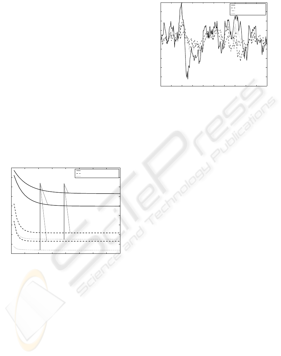
Figure 2 displays a simulated signal together with
the linear, quadratic and cubic filtering estimates for
the value p = 0.7. The result, as expected, is that the
better performance corresponds to the cubic filtering
estimate, according to the comments about Figure 1.
6 CONCLUSION
In this paper a recursive algorithm for the LS νth-
order polynomial filter and fixed-point smoother from
uncertain observations is presented, when the state-
space model of the signal is unknown. The avail-
able information is only the autocovariance and cross-
covariance functions of the signal and its Kronecker
0 20 40 60 80 100 120 140 160 180 200
−2.5
−2
−1.5
−1
−0.5
0
0.5
1
1.5
2
Time k
Signal and filtering estimates
Signal
Linear filtering estimate
Quadratic filtering estimate
Cubic filtering estimate
Figure 2: Signal and filtering estimates for p = 0.7.
powers, as well as the corresponding functions of the
additive noise. It is also assumed that the probabilities
of existence of the signal in the observed values are
available. An augmented observation equation suit-
ably defined allows us to obtain the polynomial esti-
mator of the original signal from the linear estimator
of the augmented signal.
The effectiveness of the quadratic and cubic filters
in contrast to the linear one is shown by applying the
proposed algorithm to estimate a signal generated by
a first-order autoregressive model.
ACKNOWLEDGMENT
Supported by the ‘Ministerio de Ciencia y Tec-
nolog
´
ıa’. Contract BFM2002-00932.
REFERENCES
Caballero, R., Hermoso, A. and Linares, J. (2003). Polyno-
mial filtering with uncertain observations in stochas-
tic linear systems. International Journal of Modelling
and Simulation, 23:22–28.
Magnus, J. R. and Neudecker, H. (1988). Matrix differential
calculus with applications in Statistics and Economet-
rics. Wiley & Sons, New York.
Nakamori, S., Caballero, R., Hermoso, A. and Linares,
J. (2003a). New design of estimators using covari-
ance information with uncertain observations in lin-
ear discrete-time systems. Applied Mathematics and
Computation, 135:429–441.
Nakamori, S., Caballero, R., Hermoso, A. and Linares, J.
(2003b). Second-order polynomial estimators from
uncertain observations using covariance information.
Applied Mathematics and Computation, 143:319–
338.
ICINCO 2004 - SIGNAL PROCESSING, SYSTEMS MODELING AND CONTROL
308

NaNacara, W. and Yaz, E. E. (1997). Recursive estimator
for linear and nonlinear systems with uncertain obser-
vations. Signal Processing, 62:215–228.
POLYNOMIAL ESTIMATION OF SIGNALS FROM UNCERTAIN OBSERVATIONS USING COVARIANCE
INFORMATION
309