AN EVOLUTIONARY ALGORITHM FOR IDENTIFICATION OF
NON-STATIONARY LINEAR PLANTS WITH TIME DELAY
Janusz P. Papliński
Technical University of Szczecin, Institute of Control Engineering, 26 Kwietnia 10, 71-126 Szczecin, Poland,
Keywords: evolutionary algorithm, model of dynamics, identification
Abstract. The identification of time delay in the linear plant is one of the important tasks. It is especially hard problem
when the plant is non-stationary. New possibility in this field is opened by application of an evolutionary
algorithm. The method of identification proposed in the paper is based on three classes of input signals.
In
the first case we can obtain and operate on the whole unit step response. In the second way we operate on a
random signal of control, and in the last we have the stairs input signal. The identification without and with
disturbances is considered.
1 INTRODUCTION
Some linear plants can be considered as a plant with
transport delay. The knowledge of this delay is very
important. It enables us, for example, to design an
appropriate control system. Another domain of
application of this knowledge can be in the fault
detection. If we have the possibility of indicating
changes of the time delay, we can detect faults in the
system. In this situation we can consider the above
matter as an identification of a non-stationary plant.
We need information about the changing parameters
of the plant. There are several methods of
identification of time delay and the plant dynamics
and this problem is being continuously developed
(Orlov et al., 2002). New possibility in this domain
is opened by application of evolutionary algorithms.
They include some special ability to parallel
computation of encoded information. This allows for
exploration of several promising areas of the
solution space at the same time (Goldberg, 1989
,
Michalewicz, 1996). The evolutionary algorithm
works in a periodic manner and it permits to observe
in successive iterations of changed parameters of the
identified plant.
I consider, in my paper, three classes of input
signals. In the first case we can obtain and operate
on the whole unit step response. In the second way
we operate on a random signal of control, and in the
last we have the stairs input signal. We have less
information in the each consecutive situation, and
the identification is becoming more difficult.
In my paper I considered identification of
systems without and with disturbances.
The experimental investigations take advantage
of Matlab and its “Genetic algorithm for
optimisation toolbox” (GAOT) (Houck et al. 1995a),
available from the Internet.
2 GENETIC ALGORITHMS
OPERATIONS
The genetic algorithms operate on the codable form
of individuals. Each individual sufficiently describes
the model. It is composed of 11 parameters – genes
(Papliński, 2002), coded as floating point numbers. 5
parameters correspond to coefficients of the
nominator, next 5 correspond to coefficients of the
denominator and the last one is equal to the time
delay. The obtained model corresponds to the
transfer function:
tc
e
cscscscsc
cscscscsc
sG
11
109
2
8
3
7
4
6
54
2
3
3
2
4
1
)(
−
++++
++++
=
(1)
The value of each chromosome is contained in an
assumed range. The acceptable limits are determined
on the base of the priory information about the
plant. The maximum order of models is equal to 4
and it is a compromise between accuracy and
simplicity.
64
Papli
´
nski J. (2004).
AN EVOLUTIONARY ALGORITHM FOR IDENTIFICATION OF NON-STATIONARY LINEAR PLANTS WITH TIME DELAY.
In Proceedings of the First International Conference on Informatics in Control, Automation and Robotics, pages 64-69
DOI: 10.5220/0001126800640069
Copyright
c
 SciTePress

One of the main operators of the genetic
algorithm is the operation of crossover. It is used to
create a new solution on the basis of the existing
solution. Crossover takes two individuals from old
population and produces two new individuals for the
next population. The arithmetical crossover with
random direction of changes (Papliński, 2003),
given in the form:
YaXa
XaYa
)1('Y
)1('X
−+=
−+=
(2)
where
a ∈ [-1, 1], is used in the paper
This operation is used in the investigation,
presented in the paper, with global probability of the
crossover equal approximately to 0,97.
As a selection function we use the normalized
geometric selection (Houck et al. 1995b), which
defines the probability of selection for each
individual as:
n
r
r
q
qq
p
)1(1
)1(
1
−−
−
=
−
(3)
Where:
q - the probability of selecting the best
individual;
r - the rank of individual, where 1 is the best;
n - the population size.
Individuals are graded in population according to
the quality of the obtained models. The fitness
function is obtained from differences between step
responses of the plant and models. The figure of
merit has the form
() ()()()
∑
=
−
=
200
1
2
1
i
imio
tyty
J
α
(4)
where
y
o
(t
i
) – the response of the plant;
y
m
(t
i
) – the response of the model;
α - the coefficient of importance.
The role of coefficient
α is to decrease influence
of the initial condition and it is presented in fig.1.
The identified plant works continuously all the
time during identification. In the same time for each
individual in every generation the fitness function J
is determined. The plant works with non-zero initial
conditions, the models work always with the initial
conditions equal to zero. The coefficient
α permits
to minimize the influence of initial conditions to the
fitness function J.
0
2
4
6
8
10
12
14
16
18
20
0
0.1
0.2
0.3
0.4
0.5
0.6
0.7
0.8
0.9
1
t
α
Figure 1: The value of coefficient α .
As a global quality coefficient J
g
we used the
sum of absolute error of time identifying with the
weight factor
∑
−=
identdelg
ttJ (5)
where:
t
del
- the time delay of the plant
t
ident
- the identified time delay
This figure of merit has only an experimental
application and can be used only for the simulated
plant, not for the real plant, because we do not know
the actual value of the time delay. This criteria
permit to compare evolutionary algorithms to each
other.
I used, in my investigation, the mechanism of
crowd (De Jong, 1975). The technique is employed
for insertion into the population.
Each check consists
of a randomly selected crowding sub-population
from the entire population, according to the
crowding-factor. The individuals from sub-
population are compared to the child and the child
replaces the most similar candidate on the basis of
similarity count. The similarity count
J
s
compares
individuals as follows
()
2
11
1
∑
=
−=
i
isics
ccJ
where
c
ic
– the I-th coefficient of the child;
c
is
– the I-th coefficient of the individual
from the sub-population.
This method is beneficial in that it helps to
maintain diversity throughout the search. The
diversity of population of evolutionary algorithm is
specially important for identification of the non
stationary plant. In my investigation the crowding-
factor equals 2.
AN EVOLUTIONARY ALGORITHM FOR IDENTIFICATION OF NON-STATIONARY LINEAR PLANTS WITH
TIME DELAY
65

Population is made of 80 individuals. The
genetic algorithm is terminated at the specified
generation.
2 IDENTIFICATION USING THE
UNIT STEP RESPONSE
One of the methods of identification can use the step
responses of the plant (Papliński, 2002). In this case
we need the whole unit step response in each
generation of the evolutionary algorithm. It is
possible for the slow plant drove by the step signal.
Some example of this plant, in simplification, can be
a district heating station with a pipe system.
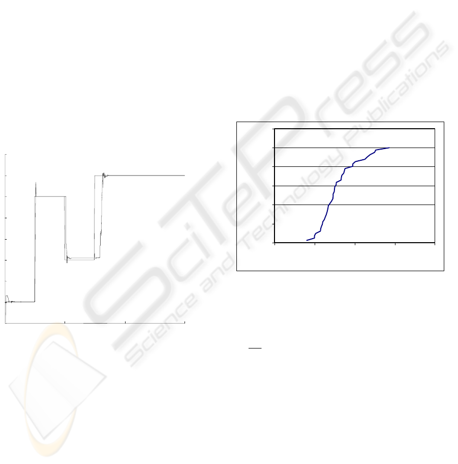
The evolutionary algorithm reads the whole step
response of the plant at the beginning of each
iteration. It permits to seek optimal solution for the
changing plant. In next steps the fitness function of
population is determined, and new population is
created. The fig.2 presents the trace of the identified
time delay for stairs changes in this time in the plant.
0
500
1000
t
[s
]
0
10
20
30
40
50
60
70
t
d
Figure 2: The trace of stairs changes in time delay of the
plant and the identified time in model.
3 ON-LINE IDENTIFICATION
USING THE TIME SIGNAL
WINDOW
The step response identification is restricted to the
small class of plants and the situation for which we
can use the step input and the complete step
response. In the majority of real systems we have
only successive samples of signal. It is possible to
do identification by using the natural signal overflow
in the identified object. The process of identification
can be made without any interfering with the plant
work. I proposed in the paper the evolutionary
algorithm operating on some sliding time signal
window. The window contains 200 following
samples of input and output signals of the plant. In
the successive generation responses of individuals
are compare to changing response of the plant.
3.1 Identification with the random
input
It seems that the most universal signal in the real
systems is random input. This class of signals
appears often in systems. Another advantage of it is
continuously excitation the plant, what is very
important in on-line identification. Experiments to
identify time delay were made. The obtained
cumulative distribution function F(x) of the global
quality coefficient
J
g
is presented in fig.3.
0,00
0,20
0,40
0,60
0,80
1,00
1,20
0,00 0,50 1,00 1,50 2,00
Jg
F(Jg)
Figure 3: The cumulative distribution function of the
global quality coefficient
J
g
.
The expected value of the global quality
coefficient with the 95 percentage of confidence
interval is equal to
07,079,0 ±=
g
J
.
The standard deviation of the obtained solution is
equal to
23,0
=
σ
. About 20% of identification has
.
1≥
g
J
Fig.4 and Fig.5 present the trace of the
identifying time delay for the average and the worst
identification. Even the worst identification
guarantees correct identification of the time delay,
but only time of identification can be longer.
ICINCO 2004 - INTELLIGENT CONTROL SYSTEMS AND OPTIMIZATION
66

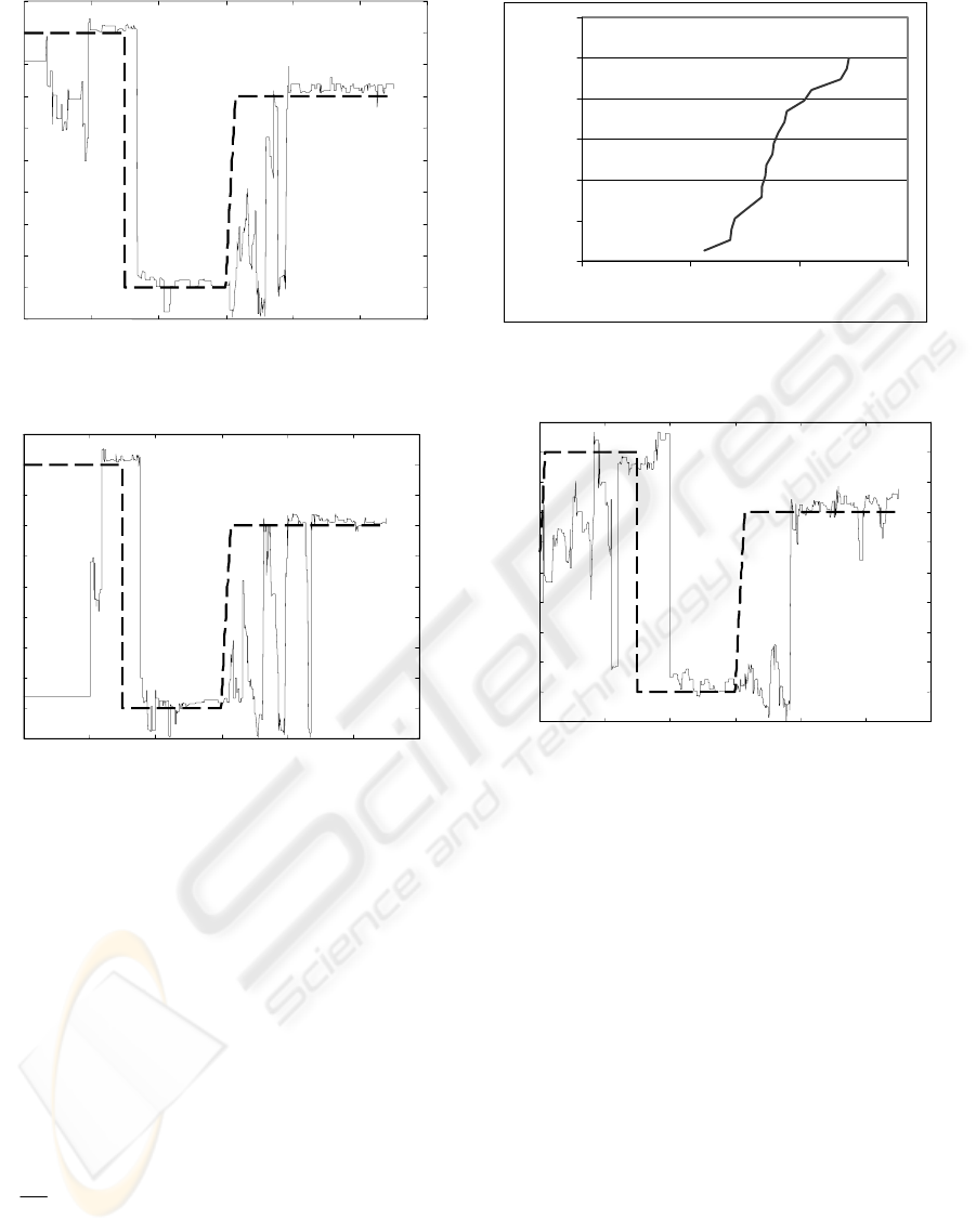
0 200 400 600 800 1000 1200
0
0.5
1
1.5
2
2.5
3
3.5
4
4.5
5
k
t
d
Figure 4: The trace of the identified time delay for the
average identification for J
g
=0.77.
0
200
400
600
800
1000
1200
0
0.5
1
1.5
2
2.5
3
3.5
4
4.5
5
k
t
d
Figure 5: The trace of the identified time delay for the
average identification for J
g
=1.47.
3.1 Identification with the stairs input
signal
Some plants can be controlled by the stairs signal. If
we want to do on-line identification the period of
sudden change cannot be too large. I made an
assumption that the average period is equal to 5. The
experiments to identify time delay were made. The
obtained cumulative distribution function of the
global quality coefficient
J
g
is presented in fig.6.
The expected value of the global quality
coefficient with the 95 percentage of confidence
interval is equal to
08,09,0 ±=
g
J
.
The standard deviation of the obtained solution is
equal
19,0=
σ
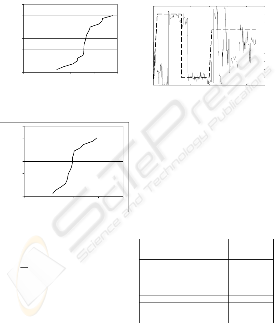
. Fig.7 presents the trace of the
identified time delay for the worst identification
obtained during the experiment..
0,00
0,20
0,40
0,60
0,80
1,00
1,20
0,00 0,50 1,00 1,50
Jg
F(Jg)
Figure 6: The cumulative distribution function of the
global quality coefficient
J
g
.
0
200
400
600
800
1000
1200
0
0.5
1
1.5
2
2.5
3
3.5
4
4.5
5
k
t
d
Figure 7: The trace of the identified time delay for the
average identification for J
g
=1.23 and the plant driven by
stairs.
The identification with the stairs input signal is
effective. The expected value of the global quality
coefficient is now a little worse than in the
identification with the random input. It may be
caused by use of worse signals to identification.
4 IDENTIFICATION IN THE
PRESENCE OF RANDOM NOISE
The results of identification presented above were
made with no disturbances. However the
disturbances always occur in real systems. I made
the assumption that output of plant is measured with
random disturbances. The value of the amplitude of
disturbances was assumed at the level equal 50% of
level of output. I made the investigation for two
classes of input:
-
the random input;
-
the stairs input.
AN EVOLUTIONARY ALGORITHM FOR IDENTIFICATION OF NON-STATIONARY LINEAR PLANTS WITH
TIME DELAY
67

The obtained cumulative distribution functions
of the global quality coefficient
J
g
are presented in
fig.8 and fig.9.
0,00
0,20
0,40
0,60
0,80
1,00
1,20
0,00 0,50 1,00 1,50 2,00
Jg
F(Jg)
Figure 8: The cumulative distribution function of the
global quality coefficient J
g
for the random input with
disturbances
.
0,00
0,20
0,40
0,60
0,80
1,00
1,20
0,00 0,50 1,00 1,50 2,00
Jg
F(Jg)
Figure 9: The cumulative distribution function of the
global quality coefficient J
g
for the stairs input with
disturbances.
The expected value of the global quality
coefficient with the 95 percentage of confidence
interval:
- for the random input is equal
11,035,1 ±=
g
J
24,0=
σ
- for the the stairs input is equal
1,097,0 ±=
g
J
.
23,0=
σ
The disturbances worsen identification, but do
not do it impossible. The random input identification
is more sensitive to them. The obtained solutions are
bad. The stairs input identification is less sensitive.
The trace of the identified time delay, for its worst
identification obtained during the experiment is
presented in fig.10. This identification is worse than
identification without disturbances, but is not bad.
We should remember that this figure presents the
worst identification of several. The identification
was made for 18 times.
0
200
400
600
800
1000
1200
0
0.5
1
1.5
2
2.5
3
3.5
4
4.5
5
k
td
Figure 10: The trace of the identified time delay for the
worst identification for J
g
=1.47 and the plant drives by
stairs with 50% disturbances.
5 CONCLUSION
The investigation presented in the paper shows that
evolutionary algorithm can be used in identification
of non-stationary plants with transport delays. The
unit step responses as well as random input can be
use. In the first case the identification is more
accurate, but we need the whole step response in
every generation. The second method is less
accurate, but we also need less information about
plants and we can use a wide class of input signals.
The summary solutions, for the on-line
identification using the time signal window, are
presented in table 1.
Table 1: The summary solutions
The
Identification
with:
g
J
σ
the random
input
07,079,0
±
0,23
the random
input with
disturbances
11,035,1
±
0,24
the stairs input
08,09,0
±
0,19
the stairs input
with
disturbances
1,097,0
±
0,23
For the identification without disturbances the
best class of inputs are random signals. This
identification is however sensitive to disturbances.
ICINCO 2004 - INTELLIGENT CONTROL SYSTEMS AND OPTIMIZATION
68

The implementation of the stairs input signal extends
this method to a wider class of inputs. Additionally,
this identification is less sensitive to disturbances.
The identification with 50% disturbances shows
that evolutionary algorithm can be used in on-line
trace of the variable time delay in the non-stationary
plant.
REFERENCES
Goldberg D. 1989. Genetic Algorithms in Search,
Optimisation, and Machine Learning. Addison –
Wesley
Houck, C. R., J. A. Joines, and M. G. Kay. 1995a. Genetic
Algorithm for Optimisation Toolbox.
www.ie.ncsu.edu/mirage/
Houck, C. R., J. A. Joines, and M. G. Kay. 1995b. A
genetic algorithm for function optimisation: A Matlab
implementation. North Carolina State University
NCSU-IE Technical Report 95-09
Michalewicz Z., 1996. Genetic algorithms + Data
structures = Evolution programs. The book, Springer –
Verlag Berlin Heidelberg.
Orlov Y., Belkoura L., Richard J.P., Dambrine M., 2002.
On-line parameter identification of linear time-delay
systems. In 41st IEEE Conference on Decision and
Control. Las Vegas, Nevada USA
Papliński J.P. 2002. An evolutionary algorithm used for
identification of linear plant with time delay. MMAR,
Szczecin Poland
Papliński J.P., 2003. Non-Degenerative Evolutionary
Algorithms for Identification of the Plants With
Variable Time Delay. 14
th
International Conference on
Proces Control’03 Slovak University of Technology in
Bratislava, Štrbskė Pleso, Slovakia,
AN EVOLUTIONARY ALGORITHM FOR IDENTIFICATION OF NON-STATIONARY LINEAR PLANTS WITH
TIME DELAY
69