
Optimization of Large-scale Transport Network as a Factor of
Sustainable Development
Dmitriy Pavlov
1
a
and João Paulo Pereira
2
b
1
Kuban State Agrarian University, Krasnodar, Russia
2
Instituto Politécnico de Bragança, Bragança, Portugal
Keywords: Planning Transport Routes, Large-scale Transport Networks, Prefractal Graphs, Multi-criteria Discrete
Optimization.
Abstract: The paper investigates the problem of optimal planning of passenger and freight transportation routes in a
large-scale transport network. Optimizing the structure of the transport network and analyzing the spatial
relationships of the functioning of the infrastructure are key ways to ensure the sustainability of regional
development. It is proposed to use fractal graphs and their limited counterpart, prefractal graphs, which are
graphs with fractal properties as a model of a large-scale transport network. The mathematical formulation of
the problem is presented as a multicriteria discrete optimization problem, where the criteria are the most
significant requirements for the system. In this formulation, the problem under study becomes a multicriteria
problem of covering a prefractal graph with simple intersecting paths. The solution of the multicriteria discrete
optimization problem is constructed using special algorithms, the quality of which is estimated by
computational complexity. We have built one of the effective algorithms for optimizing the problem
according to one of the presented criteria that allows us to select the maximum paths. The common problem
of discrete multicriteria problems is to find many alternatives, but in this paper, attention is paid to finding at
least one optimal solution from many alternatives and evaluating it according to other criteria. The advantage
of using this approach using prefractal graphs is justified by a reduction in the computational complexity of
the algorithms.
1 INTRODUCTION
The task of optimal planning of passenger and freight
transportation routes is a key problem in ensuring the
efficiency of transport infrastructure (Comtois,
2013). Infrastructure is sustainable if it brings social,
economic and environmental benefits throughout its
life cycle. When solving such a problem, it is
necessary to take into account various optimization
requirements (criteria). For example, when finding
optimal routes, it is necessary to take into account not
only economic requirements, i.e., optimization of
transportation costs but also social or environmental
requirements. As a rule, in such problems, a solution
that optimizes one of the criteria is not optimal
according to other criteria, then these tasks are multi-
criteria problems. The solution to the multicriteria
problem is not one single solution, but a set of
a
https://orcid.org/0000-0002-4677-1762
b
https://orcid.org/0000-0001-9259-0308
alternatives (Cochrane, 1973). Currently, the problem
of finding a set of alternatives is poorly studied,
including for the multicriteria discrete problem in
modelling transport routes (Emelichev, 1991).
The article studies the mathematical model of the
problem of planning transport routes in a large-scale
transport network in a multi-criteria environment. It
is proposed to use prefractal graphs (Kochkarov,
1999; Skums, 2019; Kochkarov, 2004) with the
property of a «small-world» as a model of a large-
scale transport network. Prefractal graphs are used to
model the structure of large-scale complex systems,
such as the global Internet, electric networks, and
large-scale clustering of matter in the Universe
(Kochkarov, 2004; Perepelitsa 1999; Kochkarov,
2015).
In the study of any multicriteria problem, three
stages can be distinguished, each of which is a
494
Pavlov, D. and Pereira, J.
Optimization of Large-scale Transport Network as a Factor of Sustainable Development.
DOI: 10.5220/0010592904940500
In Proceedings of the International Scientific and Practical Conference on Sustainable Development of Regional Infrastructure (ISSDRI 2021), pages 494-500
ISBN: 978-989-758-519-7
Copyright
c
2021 by SCITEPRESS – Science and Technology Publications, Lda. All rights reserved

separate task. The first step is the construction of a set
of feasible solutions. The second stage consists in
isolating from the set of feasible solutions the Pare-to
optimal so-called Pareto set (Cochrane, 1973;
Emelichev, 1991). The solution is Pareto-optimal if
the value of any of the criteria can be improved only
due to the deterioration of the values of other criteria.
At the third stage, from the Pareto set, it is necessary
to choose a solution that will be implemented taking
into account the essence of the problem (Emelichev,
1991; Kochkarov 1998).
In this paper, attention is paid to finding at least
one optimal solution from a variety of alternatives.
The concept of asymptotic time complexity is used –
the behaviour of computational complexity as a
function of input size in the limit with increasing size
of the problem (Garey, 1979). For this, a polynomial
algorithm (Garey, 1979) is constructed that allows
one to single out an effective solution with an
estimate according to given criteria.
2 METHODS
2.1 Basic Concepts in Fractal and
Prefractal Graphs
Prefractal and fractal graphs are a model of structures
growing in discrete time according to the same rules
from each of its vertices. The formal reflection of
these rules is the operation of replacing a vertex by
seed, which underlies the definition of prefractal
graphs. The term seed is any connected graph 𝐻
𝑊,𝑄 . The essence of the operation vertex
replacement by seed (VRS) is as follows. In the given
graph 𝐺𝑉,𝐸, the vertex 𝑣∈𝑉 chosen for
replacement is distinguished by the set of 𝑉
𝑣
⊆
𝑉 , 𝑗 1,2,…,|𝑉
| adjacent vertices. Further, this
vertex 𝑣 and all its incident edges are removed from
the graph 𝐺 . Then each vertex 𝑣
⊆𝑉, 𝑗
1,2,…,|𝑉
| is connected by an edge to one of the
vertices of the seed 𝐻𝑊,𝑄. The vertices are
joined arbitrarily (randomly) or according to a certain
rule if necessary.
Denote the prefractal graph by 𝐺
𝑉
,𝐸
,
where 𝑉
is the set of vertices of the graph, and 𝐸
is
the set of its edges. We define it recurrently, gradually
replacing each vertex in the graph 𝐺
constructed at
the previous stage 𝑙 1,2,…,𝐿 1 each its vertex
with the seed 𝐻𝑊,𝑄. At the stage 𝑙1, the
prefractal graph corresponds to the seed 𝐺
𝐻. The
process of generating a prefractal graph 𝐺
is the
process of constructing a sequence of prefractal
graphs 𝐺
,𝐺
,…𝐺
,…,𝐺
, called a trajectory (see
Figure 1). The fractal graph 𝐺 generated by the seed
𝐻 is determined by an infinite trajectory.
Figure 1: The trajectory 𝐺
,𝐺
,𝐺
of the prefractal graph
𝐺
generated by the seed-triangle where the adjacency of
the old edges is chosen arbitrarily.
For a prefractal graph 𝐺
, edges that appear at the l-
th, 𝑙
1,2,…,𝐿 generation stage will be called edges
of rank l. The new edges of the prefractal graph 𝐺
are the edges of rank L, and all the other edges are
called the old edges.
If we remove all edges of ranks 𝑙1,2,…,𝐿𝑟
from the prefractal graph 𝐺
, we obtain the set
𝐵
,
, 𝑟 ∈ 1,2,…,𝐿 1} blocks of the r-th rank,
where 𝑖1,2,…,𝑛
is the block ordinal number.
We call block 𝐵
,
, 𝑠1,𝑛
, of the first rank of
prefractal graph 𝐺
, 𝑙1,𝐿 from the trajectory as
seed subgraph 𝑧
.
Prefractal graph 𝐺
𝐿
𝑉
𝐿
,𝐸
𝐿
is called weighted
if for each edge 𝑒
𝑙
∈𝐸
𝐿
there is a real number
𝑤𝑒
∈𝜃
𝑎,𝜃
𝑏, where 𝑙1,𝐿 is the rank
of the edge, 𝑎0, and 𝜃
.
A prefractal graph generated by one or a set of seed
multigraph (Harary, 1979) is called a prefractal
multigraph.
2.2 Discrete Multi-criteria Problem
Statement
Let weighted prefractal graph 𝐺
𝑉
,𝐸
generated by seed 𝐻𝑊,𝑄 be given. On feasible
solution set (FSS) 𝑋𝑋𝐺
𝑥, 𝑥𝑉,𝐸
,
𝐸
⊆𝐸
consisting of all kinds of coverings of
weighted prefractal graph 𝐺
by simple intersecting
paths, a vector-valued objective function (VVOF) is
defined as follows:
F𝑋
𝐹
𝑥,𝐹
𝑥,𝐹
𝑥,
Optimization of Large-scale Transport Network as a Factor of Sustainable Development
495

𝐹
𝑥,𝐹
𝑥,𝑥 ∈ 𝑋
(1
)
𝐹
𝑥 𝑤𝑒
∈
→min
(2
)
where
∑
𝑤𝑒
∈
is sum of all edges included in
covering 𝑥;
𝐹
𝑥 min
,
𝑤𝐶
→max
(3)
where 𝑤𝐶
is length of the maximal path from
covering 𝑥∈𝐶
,𝐶
,... ,𝐶
,... ,𝐶
.
𝐹
3
𝑥 𝑁𝑥 → min
(4)
where 𝑁𝑥 is number of all maximal paths in
covering 𝑥;
𝐹
𝑥 𝑖 → min
(5)
for any mixed path 𝐶
from covering 𝑥.
𝐹
𝑥 𝜌
𝑢,𝑣 𝜌
𝑢,𝑣 → min
(6)
where 𝜌
𝑢,𝑣 is the distance (between any vertices
𝑢,𝑣 ∈ 𝑉
) passing through the edges belonging to
covering 𝑥, while 𝜌
𝑢,𝑣 is the distance between
any vertices 𝑢,𝑣 ∈ 𝑉
in graph 𝐺
.
In terms of transport systems, the above criteria of
the VVOF (1)-(6) have a certain meaningful
interpretation (Comtois, 2013). The weights of the
edges of the prefractal graph 𝐺
may correspond to
certain costs and restrictions when moving vehicles
along the nodes of the transport network. Criterion (2)
factors in the costs incurred by passengers and the
authorities that are managing the transport system.
During operation, costs should be minimal.
Optimization by criterion (3) allows you to find
routes containing the largest number of nodes in your
path. Optimal for this criterion is a coating containing
maximum paths. To get to the desired node of the
transport network with the least number of transfers,
it is necessary to reduce the total number of routes in
the system; for this purpose, criterion (4) is used.
Important features of the transport system are the
locality and differentiation of its routes. Intra-regional
(city, intra-district) should be transport routes of
shorter length and less weight, thereby ensuring
locality. This simplifies the process of administering
the transport system at a certain level (district, city,
etc.). Interregional routes are longer and with more
weight. Differentiation refers to the separation of
routes according to their functions into inter-regional
and intra-regional. At the intersection of intra-
regionality and inter-regionality, a violation of
differentiation may occur, i.e., deterioration in the
functionality of the route. Criterion (5) is responsible
for preventing such situations in the operation of the
transport system in the VVOF (1)-(6). Mixed path 𝐶
is a route model combining both functions – intra-
regional and inter-regional – since its old edges
connect the blocks and seed subgraphs of prefractal
graph 𝐺
, which correspond to the maps of the roads
of districts, cities, etc. When operating a transport
system, it is often required that the final destination
will be reached with the least number of stops.
Criterion (6) reflects these requirements on
construction of such routes.
3 RESULTS
3.1 The Algorithm for Finding the
Largest Maximum Paths
The 𝛽
algorithm finds covering 𝑥
𝐽𝑉
,
𝐸
𝐶
,𝐶
,... ,𝐶
,... ,𝐶
∈𝑋 on prefractal
graph, where all 𝐶
𝑣
,𝑢
paths are simple, 𝑘
1,𝐾
. 𝛽
is based on the largest maximal path finding
algorithm (LMPF algorithm) on an arbitrary graph.
Using the LMPF algorithm as a procedure, the 𝛽
algorithm finds subgraph 𝐽
𝑉
,𝐸
𝐶
,
𝐶
,... ,𝐶
,... ,𝐶
on each seed subgraph of set
𝑍𝐺
∈𝑧
,𝑙1,𝐿, 𝑠1,𝑛
of prefractal graph
𝐺
such that all paths 𝐶
𝑢,𝑣 are maximal (i.e.
|
𝐶
|
min), 𝑘1,𝐾
, among all paths between
vertices 𝑢,𝑣 ∈ 𝑉
of seed subgraph 𝑧
and the
largest. Set of coverings 𝐽
,𝑙1,𝐿, 𝑠1,𝑛
,
selected on seed subgraphs of prefractal graph 𝐺
,
forms covering 𝑥
𝐽𝑉
,𝐸
.
3.1.1 LMPF Algorithm
INPUT: graph 𝐺𝑉,𝐸.
OUTPUT: spanning subgraph 𝐽𝑉,𝐸
𝐶
,𝐶
,
... ,𝐶
,... ,𝐶
.
STEP
1. Find set 𝐶′
,𝐶′
,... ,𝐶′
,... ,𝐶′
of all shortest paths between each pair of vertices
𝑢,𝑣 ∈ 𝑉 of graph 𝐺 . From 𝐶′
,𝐶′
,... ,𝐶′
,
... ,𝐶′
remove all those paths that are completely
contained in others. Combine the remaining ones into
set 𝐶
,𝐶
,... ,𝐶
,... ,𝐶
∗
, assigning them
indices such that the length of the 𝑖
-th path is not
greater than the length of the 𝑖
-th path, 𝑘1,𝐾
∗
.
Consider paths 𝑢,𝑣 and 𝑣,𝑢 for any pair of
ISSDRI 2021 - International Scientific and Practical Conference on Sustainable Development of Regional Infrastructure
496

vertices 𝑢,𝑣 ∈ 𝑉 as identical and include only one of
them in set 𝐶
,𝐶
,... ,𝐶
,... ,𝐶
∗
. Set 𝐶
,𝐶
,
...,𝐶
,... ,𝐶
∗
is a set of maximal paths of graph
𝐺, where 𝐶
is the diametral path.
STEP 2. Cover the vertices and edges of graph 𝐺
with paths from set 𝐶
,𝐶
,... ,𝐶
,... ,𝐶
∗
sequentially, starting with the 𝑖
-th. For the covering
of graph 𝐺 with path 𝐶
, we will have in mind
selection of vertices and edges forming the 𝐶
. path
on graph 𝐺 . We use only paths that satisfy the
condition that each new path selects at least one other
vertex of graph 𝐺that is not covered by previous
paths.
STEP
3. Assign numbers (in the order they are
used) to all paths from set 𝐶
,𝐶
,... ,𝐶
,
... ,𝐶
∗
used to cover vertices and edges of graph
𝐺. Cover graph until there are no unselected vertices
left.
STEP
4. Set of paths 𝐶
,𝐶
,... ,𝐶
,... ,𝐶
⊆
⊆𝐶
,𝐶
,... ,𝐶
,... ,𝐶
∗
, used to cover graph
𝐺, form the desired covering 𝐽𝑉,𝐸
𝐶
,𝐶
,
... ,𝐶
, consisting of the largest maximal paths
𝐶
𝑣
,𝑢
𝑘1,𝐾
.
Theorem 1.
The computational complexity of the
LMPF algorithm that finds covering 𝐽𝑉,𝐸
on
graph 𝐺 𝑉, 𝐸,
|
𝑉
|
𝑛, is 𝑂𝑛
.
P
ROOF. Finding the shortest distance between any
two vertices of graph 𝐺 will take no more than 𝑛
simple operations. In its first step, the LMPF
algorithm finds all the shortest paths of graph 𝐺, and
they are equal to 𝑛𝑛 1/2 𝑛
in number. Next,
the algorithm selects (by comparing the paths) some
part of these paths. Since all the vertices and edges
that make up the paths are known, comparing the
paths will take 𝑛
operations. In total, the
computational complexity of the LMPF algorithm is
𝑂𝑛
𝑛
𝑛
𝑂𝑛
.
3.1.2 The 𝜷
𝟐
Algorithm
INPUT: prefractal graph 𝐺
𝑉
,𝐸
.
OUTPUT: connected spanning subgraph 𝐽
𝑉
,𝐸
𝐶
,𝐶
,... ,𝐶
,... ,𝐶
.
STEP 1. Construct a set of seed subgraph 𝑍𝐺
𝑧
, 𝑙1,𝐿, 𝑠1,𝑛
for prefractal graph 𝐺
.
In accordance with constructed set 𝑍𝐺
, number all
the edges of prefractal graph 𝐺
.
STEP 2. One at a time, in a decreasing order of rank
𝑙𝐿,𝐿1,...,2,1 find spanning subgraphs 𝐽
𝑉
,𝐸
𝐶
,𝐶
,... ,𝐶
on all seed
subgraphs 𝑧
, 𝑠1,𝑛
, from set 𝑍𝐺
, using the
LMPF algorithm. After finding 𝐽
𝑉
,
𝐸
, 𝑠1,𝑛
, create set of paths 𝐶
∗
𝐶
,
,
𝐶
,
,... ,𝐶
,
,... ,𝐶
,
𝐽
𝑉
,𝐸
.
Further, each time after path set 𝐶
∗
𝐶
,
,𝐶
,
,... ,𝐶
,
,... ,𝐶
,
,
𝑙𝐿,𝐿1,... ,2,1, is created, connect each of its
𝐶
,
paths to the edges of the paths of seed
subgraphs 𝑧
and combine them into a new path
set 𝐶
∗
as follows.
STEP 3. Attach any edge ∈𝐶
𝑣
,𝑢
, 𝑘
1,𝐾
, of path 𝐶
∈𝐽
of seed subgraph 𝑧
,
𝑠1,𝑛
, to that path from set 𝐶
∗
, to which it
is incident at the end. The path formed in this way is
introduced into a new path set 𝐶
∗
.
If edge 𝑒 is incident to one of its ends by several
paths from𝐶
∗
, then all the paths formed in this
case are introduced into set 𝐶
∗
. If both vertices
𝑣
,𝑢
of edge 𝑒 are incident to the ends of two
different paths 𝐶
,
and 𝐶
,
respectively,
then a path formed by paths 𝐶
,
, 𝐶
,
and
edge 𝑒 is added to set 𝐶
∗
only if the ends of
paths 𝐶
,
and 𝐶
,
that are not incident to
edge 𝑒are also not incident to the ends of other paths
from 𝐶
∗
. Otherwise, add the paths formed by
several paths from 𝐶
∗
and several edges of the
paths of seed subgraphs of 𝑙 1-th rank to set
𝐶
∗
.
If edge 𝑒 is not incident to any paths of 𝐶
∗
,
then insert it into set 𝐶
∗
as a separate path.
STEP 4. At the input of the previous step, after the
paths of all seed subgraphs have been processed, a set
of paths 𝐶
∗
𝐶
,
,𝐶
,
,... ,𝐶
,
,... ,𝐶
,
will
be obtained. Set of paths 𝐶
,𝐶
,...,𝐶
,...,𝐶
obtained from 𝐶
∗
by changing the numbering
defines the required spanning subgraph 𝐽𝑉
,𝐸
.
Theorem 2. The 𝛽
algorithm finds connected
spanning subgraph 𝐽𝑉
,𝐸
𝐶
,𝐶
,... ,𝐶
,
... ,𝐶
, where 𝐶
are simple paths, on prefractal
graph 𝐺
𝑉
,𝐸
, generated by seed 𝐻𝑊,
𝑄,
|
𝑊
|
𝑛.
The proof of the theorem is based on the design
features of the construction of prefractal graphs and
the operation of the algorithm 𝛽
.
Theorem 3. The computational complexity of the
𝛽
algorithm that selects covering 𝐽𝑉
,𝐸
on
prefractal graph 𝐺
𝑉
,𝐸
, generated by seed
𝐻𝑊,𝑄, where
|
𝑊
|
𝑛,
|
𝑉
|
𝑁𝑛
, is
equal to 𝑂𝑁𝑛
.
Optimization of Large-scale Transport Network as a Factor of Sustainable Development
497

Proof. The 𝛽
algorithm is essentially a multiple
execution of step 2. Step 2, in turn, is a multiple
invocation to the LMPF algorithm, whose
computational complexity is equal to 𝑂𝑛
. Since
the 𝛽
algorithm invokes the SPS (shortest path
selection) algorithm 𝑘
times, it will perform
no more than 𝑘⋅𝑂𝑛
operations.
Then, 𝑂𝑘 ⋅𝑛
𝑂
⋅𝑛
𝑂𝑛
⋅𝑛
𝑂𝑁𝑛
.
Hence, the computational complexity of the 𝛽
algorithm is equal to 𝑂𝑁𝑛
.
Theorem 4. The 𝛽
algorithm selects covering
𝑥
𝐽𝑉
,𝐸
𝐶
,𝐶
,...,𝐶
,...,𝐶
∈𝑋,
where 𝐶
are the shortest paths of same rank, on
prefractal graph 𝐺
𝑉
,𝐸
generated by seed
𝐻𝑊,𝑄,
|
𝑊
|
𝑛,
|
𝑄
|
𝑞, estimated by the
first criterion:
𝐹
𝑥
∈𝑎
𝑛1
/
;𝑞𝑏
/
.
Proof. Covering 𝑥
𝐽𝑉
,𝐸
𝐶
,𝐶
,
... ,𝐶
,... ,𝐶
selected by the 𝛽
algorithm on
prefractal graph 𝐺
generated by seed, belongs to
feasible solution set 𝑋 of vector-valued objective
function (1)-(6).
We first establish the upper bound of the estimate.
The 𝐹
𝑥 criterion is weighted and its value is equal
to the sum of the weights assigned to the edges of
covering 𝑥∈𝑋. Obviously, the covering from the
feasible solution set consisting of all edges of
prefractal graph 𝐺
will have the greatest weight, i.e.,
when 𝑥𝐺
. Using the prefractal graph weighting
rule, we give an estimate of the total weight 𝑤𝐺
of
prefractal graph 𝐺
. We denote the total weight of
seed subgraph 𝑧
∈𝑍𝐺
of rank 𝑙, 𝑙1,𝐿 under
serial number 𝑠 , 𝑠1,𝑛
as 𝑤𝑧
, then
𝑤𝐺
∑∑
𝑤𝑧
. The weight of a single seed
of rank 𝑙, 𝑙1,𝐿
is estimated as 𝑤𝑧
𝑞𝑎/
𝑏
𝑏, where
|
𝑄
|
𝑞 is the number of edges in seed
𝐻. Accordingly, the sum of the weights of all same-
rank seed subgraphs of prefractal graph 𝐺
is limited
by inequality
∑
𝑤𝑧
𝑞𝑏𝑎/𝑏
𝑛
. As a
result, the weight of the prefractal graph is limited as
𝑤𝐺
∑
𝑞𝑏𝑎/𝑏
𝑛
𝑞𝑏
/
/
.
We now establish the lower bound of the estimate.
The smallest (by weight) covering from the feasible
solution set should be some spanning tree of
prefractal graph 𝐺
. To get the lower bound of the
estimate by the first criterion, we only need to
estimate the weight of the minimum spanning tree
(Swamy, 1983) 𝑇𝑉
,𝐸
selected on prefractal
graph 𝐺
. Each edge of seed subgraph 𝑧
of rank 𝑙,
according to the prefractal graph weighting rule,
cannot be less than 𝑎/𝑏
𝑎. Then 𝑤𝑇
𝑛
1𝑎/𝑏
𝑎, where 𝑛 1 is the number of edges
of any spanning tree, while the total weight of the
minimum spanning tree of the seed subgraph of same
rank is
∑
𝑤𝑇
𝑎𝑛 1𝑎/𝑏
𝑛
, 𝑙
1,𝐿
. For the weight of minimum spanning tree 𝑇, the
following inequality holds: 𝑤𝑇
∑
𝑎𝑛1𝑎/
𝑏
𝑛
𝑎𝑛1
/
/
.
Thus, the value of function 𝐹
𝑥
, from the
covering constructed by the 𝛽
algorithm falls within
the interval
𝐹
𝑥
∈𝑎𝑛1
/
/
;𝑞𝑏
/
/
.
Theorem 5. The 𝛽
algorithm selects connected
spanning subgraph 𝐽𝑉
,𝐸
𝐶
,𝐶
,... ,𝐶
,
... ,𝐶
, where 𝐶
are the shortest paths, on
prefractal graph 𝐺
𝑉
,𝐸
generated by seed
𝐻𝑊,𝑄,
|
𝑊
|
𝑛,
|
𝑄
|
𝑞, for which the
adjacency of its old edges is not violated.
Proof. We define the operation of “gluing” together
two arbitrary graphs 𝐺′ 𝑉′, 𝐸′ and 𝐺′′
𝑉′′,𝐸′′. Two vertices – 𝑣′ ∈ 𝑉′ and 𝑣′′ ∈ 𝑉′′ – are
selected for merging. Graph 𝐺
𝑉
,𝐸′ ∪ 𝐸′′ ,
derived from graphs 𝐺′ and 𝐺′′ by merging vertices
𝑣′ and 𝑣′′ into some vertex 𝑣∈𝑉
such that all edges
incident to vertices 𝑣′ and 𝑣′′ become incident to
vertex 𝑣, is called glued from graphs 𝐺′ and 𝐺′′.
Prefractal graph 𝐺
𝑉
,𝐸
, generated by seed
𝐻 𝑊, 𝑄, such that the adjacency of its old edges
in the generation process is not violated. Then,
prefractal graph 𝐺
can be obtained by gluing
together all
seed subgraphs 𝑍𝐺
𝑧
, 𝑙
1,𝐿
, 𝑠1,𝑛
(Kochkarov, 1998). First, first-rank
seed subgraph 𝑧
is glued at each of its vertices with
second-rank seed subgraph 𝑧
, 𝑠1,𝑛. Further,
each prefractal graph 𝐺
generated in this way at the
𝑙-th step, 𝑙1,𝐿1
, is glued at each of its vertices
with seed subgraphs 𝑧
, 𝑠1,𝑛
. As a result,
we obtain prefractal graph 𝐺
at the 𝐿-th step of
which the adjacency of its old edges is not violated.
If connected spanning subgraphs 𝐷
, 𝑙1,𝐿, 𝑠
1,𝑛
are selected on all seed subgraphs 𝑧
of
prefractal graph 𝐺
, then graph 𝐷 obtained by
gluing together graphs 𝐷
, similarly to generation
of graph 𝐺
described above, will become the
spanning subgraph of graph 𝐺
. This will happen due
to the mutual correspondence of the edge numbers of
ISSDRI 2021 - International Scientific and Practical Conference on Sustainable Development of Regional Infrastructure
498
seed subgraphs 𝑧
, participating in the generation
of graphs 𝐷 and 𝐺
.
The 𝛽
algorithm selects a spanning subgraph
𝐽
𝑉
,𝐸
, consisting of a set of simple
shortest paths 𝐶
,𝐶
,... ,𝐶
,... ,𝐶
. on each
seed subgraph 𝑧
∈𝑍𝐺
, 𝑙1,𝐿, 𝑠1,𝑛
of
prefractal graph 𝐺
𝑉
,𝐸
.
Recall that all paths 𝐶
,𝐶
,... ,𝐶
,... ,𝐶
forming covering 𝐽𝑉
,𝐸
are either paths of
coverings 𝐽
𝑉
,𝐸
, 𝑙1,𝐿, 𝑠1,𝑛
,
or consist of paths of these coverings. In both cases,
all the paths are the shortest. In the first case, the paths
are shortest thanks to the LMPF algorithm, and in the
second, this is a consequence of the special way of
defining prefractal graph 𝐺
(the adjacency of its old
edges is not violated).
Thus, covering 𝐽𝑉
,𝐸
consists of many
simple paths 𝐶
,𝐶
,... ,𝐶
,... ,𝐶
, and each
path 𝐶
𝑘
𝑣
𝑘
,𝑢
𝑘
is the shortest 𝑘1,𝐾, among
all possible paths between vertices 𝑣
𝑘
,𝑢
𝑘
∈𝑉
𝐿
of
prefractal graph 𝐺
𝐿
.
4 DISCUSSION
The proposed mathematical model of a large-scale
transport network is based on the apparatus of the
theory of fractal graphs (Kochkarov, 1998). Let L be
the rank of the simulated system, which can
correspond to a certain level of the hierarchical
structure of the administrative-territorial
administration of the region (Comtois, 2013). The
mathematical model of the road map is constructed in
the form of the trajectory of a prefractal graph
generated by a seed set 𝛨𝐻
,𝐻
,...,𝐻
,...,𝐻
.
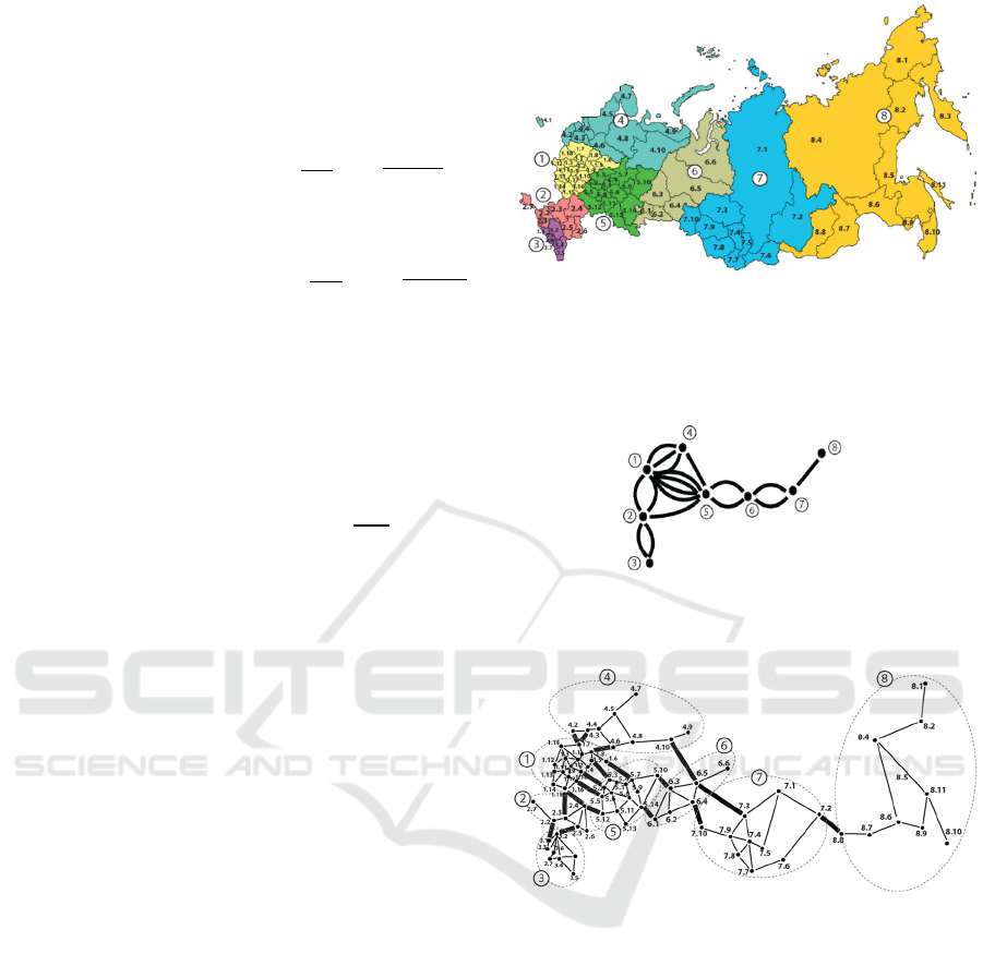
Consider the process of building a transport network
using the example of Russian roads. Geographically,
Russia consists of 8 federal districts (see Figure 2). At
the first stage, the 𝐺
𝐻
seed is a multigraph in
which the federal roads correspond to the edges and
the federal districts correspond to the vertices (see
Figure 3). Further, in 𝐺
, each vertex is replaced by a
seed corresponding to the regions within the federal
district. The structure obtained in the second stage
corresponds to the prefractal graph 𝐺
(see Figure 4).
In the next step, each vertex is replaced by a set of
seeds, corresponding to regional or municipal
districts. This process continues until the necessary
level of hierarchy of the system under study is
reached.
Figure 2: An example of a two-level hierarchy of the
territorial division of the Russian Federation is presented.
Eight federal districts of the Russian Federation designated
1-8, which consist of 85 constituent entities of the Russian
Federation.
Figure 3: The
𝐺
multigraph is presented, where the federal
districts correspond to the vertices, and the federal roads
correspond to the edges.
Figure 4: The prefractal graph
𝐺
of rank
𝐿=2
is obtained
from the multigraph
𝐺
, in which each vertex is replaced by
seeds corresponding to the structure of roads between the
federal subjects belonging to the federal district. Bold edges
are edges of rank 𝐿1 (federal highways), the remaining
edges belong to rank 𝐿2 (roads of federal subjects).
As the whole system of transport routes, we took the
coverage of the prefractal graph consisting of paths
corresponding to some routes. All necessary
requirements and restrictions imposed on routes are
expressed as a vector-valued objective function.
The use of prefractal graphs as a model of a large-
scale transport network can significantly reduce the
computational complexity of algorithms for finding
optimal solutions. Comparing the computational
complexity of the LMPF and 𝛽
algorithms on
prefractal graph 𝐺
, we obtain 𝑂𝑁
𝑂𝑁𝑛
.
Optimization of Large-scale Transport Network as a Factor of Sustainable Development
499

Therefore, the computational complexity of 𝛽
is
𝑛
times less than the computational complexity of
the LMPF algorithm.
It is worth noting that it is convenient to construct
parallel algorithms on prefractal graphs.
5 CONCLUSIONS
In the article, an approximate algorithm was used,
which is called the algorithm with estimates. The
search for efficient and accurate methods for many
NP-hard or intractable problems has no practical
sense. In this situation, we are forced either to proceed
to the study of more particular problems and to search
for low-laborious algorithms for them, or to build
approximate algorithms. This gives rise to an
approach to algorithmic problems, which is called
"algorithms with estimates". We are talking about a
vector assessment of the quality of algorithms.
Criteria, i.e. the components of this vector function
(i.e., estimates) are computational complexity,
accuracy, memory size, size of the region within
which the desired solution (many alternatives) is
almost always obtained at the output of the algorithm,
etc.
The constructed model and the algorithm for
allocating maximum routes in terms of inclusion
makes it possible to effectively solve the problem of
route planning in large-scale transport networks.
REFERENCES
Cochrane, J. L. and Zeleny M. (1973). Multiple Criteria
Decision Making, Columbia, South Carolina:
University of South Carolina Press.
Comtois, C., Slack, B. and Rodrigue, J.-P. (2013). The
geography of transport systems, Routledge, Taylor &
Francis Group, London, 3
rd
edition.
Emelichev, V. A. and Perepelitza, V. A. (1991). Complex
of vector optimization problems on graphs.
Optimization, 22(6): 903-918.
Garey, M. R. and Johnson, D. S. (1979). Computers and
Intractability: A Guide to the Theory of NP-
Completeness, New York: W.H. Freeman.
Harary, F. (1969). Graph Theory, Reading, Massachusetts:
Addison-Wesley.
Kochkarov A. A. and Kochkarov R. A. (2004). A parallel
algorithm for searching for the shortest path on
prefractal graphs. Computational Mathematics and
Mathematical Physics, 44(6): 1088‑1092.
Kochkarov A. A., Kochkarov R. A. and Malinetskii G. G.
(2015). Issues of dynamic graph theory. Computational
Mathematics and Mathematical Physics, 55(9): 1590–
1596.
Kochkarov, A. and Perepelitsa V. (1998). Fractal Graphs
and Their Properties. In ICM’98, International
Congress of Mathematicians.
Perepelitsa, V. A., Sergienko, I. V. and Kochkarov, A. M.
(1999). Recognition of fractal graphs. Cybern Syst Anal
35(4): 572–585.
Skums, P. and Bunimovich L. (2019). Graph fractal
dimension and structure of fractal networks: a
combinatorial perspective.
Swamy, M. N. S. and Thulasiraman, K. (1981). Graphs,
Networks, and Algorithms. Wiley.
ISSDRI 2021 - International Scientific and Practical Conference on Sustainable Development of Regional Infrastructure
500
