Applying Machine Learning to Weather and Pollution Data Analysis for

a Better Management of Local Areas: The Case of Napoli, Italy

Lelio Campanile

, Pasquale Cantiello

, Mauro Iacono

, Roberta Lotito

Fiammetta Marulli

and Michele Mastroianni

Dipartimento di Matematica e Fisica, Universit

a degli Studi della Campania ”L. Vanvitelli”, viale Lincoln 5, Caserta, Italy

Osservatorio Vesuviano, Istituto Nazionale di Geoﬁsica e Vulcanologia, via Diocleziano 328, Napoli, Italy

pasquale.cantiello@ingv.it

Keywords:

Air Quality, Forecasting, Machine Learning, Regression, Data Analysis, Campania.

Abstract:

Local pollution is a problem that affects urban areas and has effects on the quality of life and on health

conditions. In order to not develop strict measures and to better manage territories, the national authorities

have applied a vast range of predictive models. Actually, the application of machine learning has been studied

in the last decades in various cases with various declination to simplify this problem. In this paper, we apply

a regression-based analysis technique to a dataset containing ofﬁcial historical local pollution and weather

data to look for criteria that allow forecasting critical conditions. The methods was applied to the case study

of Napoli, Italy, where the local environmental protection agency manages a set of ﬁxed monitoring stations

where both chemical and meteorological data are recorded. The joining of the two raw dataset was overcome

by the use of a maximum inclusion strategy as performing the joining action with ”outer” mode. Among the

four different regression models applied, namely the Linear Regression Model calculated with Ordinary Least

Square (LN-OLS), the Ridge regression Model (Ridge), the Lasso Model (Lasso) and Supervised Nearest

Neighbors Regression (KNN), the Ridge regression model was found to better perform with an R

(Coefﬁcient

of Determination) value equal to 0.77 and low value for both MAE (Mean Absolute Error) and MSE (Mean

Squared Error), equal to 0.12 and 0.04 respectively.

1 INTRODUCTION

Since the beginning of the Industrial Revolution, one

of the most affected environmental sector is the air:

indeed, exhausted gases from human activities have

changed the local atmosphere composition and this

variation led to a relationship change between human

and local area. It is an instilled thought that near in-

dustrial area or even in high urbanization area the air

quality is poor, while, in order to ’breathe fresh air’,

it is necessary to go to a natural place like seafront

or mountains. As matter of fact, the connection be-

tween the presence of some compounds, their con-

centration and the onset of speciﬁc disease is widely

studied. The direct consequences is the different use

of the territory with economic implication.

The natural atmospheric composition is well

known: nitrogen accounts for 78%, oxygen 21% and

argon 0.9%. Gases like carbon dioxide, nitrous ox-

ides, methane, and ozone are trace compounds that

account for about a tenth of one percent of the atmo-

sphere. The presence and concentration of the trace

gases can be characteristic for particular area (vol-

canic areas with the presence of hydrogen sulphide,

rice paddies with methane presence): the variation

of these compounds, both qualitatively and quantita-

tively, from their standard presence is called pollu-

tion. Actually, in consideration of the human activi-

ties and aerial transport/dispersion, it is nearly impos-

sible to ﬁnd a location on Hearth unpolluted. How-

ever, it is clear that the pollution from a city center is

different compared both to an industrial area and to

a local mountain village. In addition, even between

two similar cities, the atmospheric pollution can be

completely different due to meteorological asset, city

architecture, regional location. Generally, we can say

that the air quality depends on two classes of inﬂu-

ence: the ﬁrst regards the natural condition such as

local weather, presence of water body, presence of

emitting geological structures and so on. The sec-

ond class regards the human-effect presence and so

354

Campanile, L., Cantiello, P., Iacono, M., Lotito, R., Marulli, F. and Mastroianni, M.

Applying Machine Learning to Weather and Pollution Data Analysis for a Better Management of Local Areas: The Case of Napoli, Italy.

DOI: 10.5220/0010540003540363

In Proceedings of the 6th International Conference on Internet of Things, Big Data and Security (IoTBDS 2021), pages 354-363

ISBN: 978-989-758-504-3

it is related to all the human activities that emit in the

atmosphere. Looking at a micro-scale area, new fac-

tors can be added: for example, the city architecture

can inﬂuence the wind direction and speed resulting

in different dispersion scenario or the implementation

of a green area can decrease local contamination.

In order to restrain the continuous pollution and to

try restoring some area to a better status, worldwide

regulations have been issued: most of them imposed

concentration limits both for outdoor air regarding

pollutants like carbon monoxide, BTEX (Benzene

- Toluene - Ethylbenzene - Xylene), nitrogen ox-

ides, particular matter, and limit for speciﬁc emitting

sources as industrial plants and human activities with

the use of organic solvents. The overall strategy is to

limit the emitting source where and when it is possi-

ble, and to check the air quality as result of the previ-

ous described factor. With the collected data, logged

from stationary and mobile station, there is the pos-

sibility to assess the air quality by the use of some

indicators based on the detected concentration of spe-

ciﬁc pollutant. A similar indicator is used in Europe,

namely European Air Quality Index (EAQI), as estab-

lished by 2008/50/CE directive. The hourly index is

based on concentration values for up to ﬁve key pollu-

tants and it reﬂects the potential impact of air quality

on health, driven by the pollutant for which concen-

trations are poorest due to associated health impacts.

The data are collected by stationary stations managed

by local authorities.

In Italy, the transposition of the European di-

rective took place with the enactment of law D.lgs.

155/2010 that has established a uniﬁed regulatory

framework for the assessment and management of

ambient air quality. Regions are assigned the respon-

sibility to assess this quality, to classify the regional

territory into zones and agglomerations, and to draw

up plans and programs to maintain ambient air quality

where it is good and to improve it in other cases. The

national law imposes limits to outdoor pollutants con-

centration and, since the private transport sector has

been identiﬁed as the major contributor to city pollu-

tion, in case of exceeding daily limits, the city admin-

istration restricts the access for private transport.

In this scenario, the implementation of forecasting

modeling systems have become increasingly impor-

tant in order to understand the future impacts of the

human activities and to manage local areas. Forecast-

ing can both be applied to the new emitting sources

in order to understand their relative impact on local

air, and directly to outdoor air quality to understand

its development. It is clear that in the ﬁrst case the

problem resolution is easier since all the factors that

affect the ﬁnal result are well known (characteristics

of the emitting source, pollutant concentration, plant

layout, etc.). In the second case, the factors that took

part in the game are various and not always so well

deﬁned: indeed, the local impact detected by station-

ary stations is due to a series of events such as par-

ticular wind direction, local trafﬁc, presence of a new

apartment blocks and so on. Hence, in the situation of

a micro-scale forecasting, the boundary between the

inﬂuence classes for the air quality is very blurred. To

help solve this problem, the use of machine learning

techniques seems to be a promising practice.

In the last years, many scholars have studied the

implementation of forecasting modeling with ma-

chine learning: the results may signiﬁcantly vary, de-

pending on the used dataset and the implementation

made. The machine learning help is based on the as-

sumption of a black box mechanism for the air qual-

ity: the forecast is essentially based on the ’training’

on a speciﬁc dataset, which results in the extrapola-

tion of a statistical set of rules that can be applied to

the newly collected data. Globally, the shown trends

indicate an improvement in the forecast on an ex-

tended area, such as a region, or at national level, with

high level datasets. The forecast buffer time can also

vary according to the used mechanism.

In this paper, an application of a forecasting mod-

eling approach implemented by a machine learning

based technique is presented for an Italian city where

air quality is assessed by means of stationary stations

controlled by local authorities according to D.lgs.

155/2010. The aim of this research is to understand

if this application can lead to a good forecast on a

focused area with a few analyzing stations and local

weather stations in order to better manage the area be-

fore the limits imposed are exceeded. The main origi-

nal contribution is the application of this kind of anal-

ysis on combined ofﬁcial pollution and weather data

about Campania region: at the best of our knowledge,

no such analysis is available in literature. In addition,

at the moment as per practice the data collected from

the station are ﬁrstly validated by a third part before

they are used for forecasting purposes. Indeed, this

quality check and assurance (QC/QA) is an essential

phase and it is usually handmade by few technicians.

For these reasons, it could easily be affected by errors

and hence data loss. Consequently, for this research

we only used raw data in order to check how they per-

form without any preliminary screening.

After this section, the paper is organized as fol-

lows: next section presents related work, and a brief

background on this ﬁeld is summarized; then the

case study and the used dataset are described; sub-

sequently, the methodology used to develop the fore-

casting model by means of machine learning; results

Applying Machine Learning to Weather and Pollution Data Analysis for a Better Management of Local Areas: The Case of Napoli, Italy

355

and discussion close the paper, together with future

work and developments.

2 RELATED WORKS

Several type of forecasting methods have been dis-

cussed in literature, regardless of a speciﬁc context as

in (Chatﬁeld, 2000) or (Hyndman and Athanasopou-

los, 2018). Forecasting methods can be in general di-

vided into three main categories: those that only deal

with expert opinion, those based on physical models

(Brandt et al., 2001), and those that instead make pre-

dictions based on a statistical analysis of values in a

series (Armstrong, 2001).

A discussion based on published reviews and re-

cent analyses about challenges, applications and ad-

vances, main gaps and trends along with research

needs for atmospheric composition and air quality

modeling and forecasting can be found in (Baklanov

and Zhang, 2020).

A model to predict emission concentrations of

, SO

, O

for a selected number of forward time

steps is proposed in (Doma

nska and Wojtylak, 2014)

and named e-APFM. It requires large historical data

series for weather forecast, meteorological and pol-

lution data enriched with information about the wind

direction in sectors and meteorological stations.

Wind strength and direction is a key feature in

the propagation of pollutants. In (Contreras and

Ferri, 2016) several regression models have been

compared to be able to predict the levels of four dif-

ferent pollutants (CO, NO

, SO

, O

) in several lo-

cations of a city. Different techniques to incorporate

wind strength and direction in the regression models

have been studied and applied within an interpolation

method.

A recent review on the intelligent modeling strate-

gies in the air quality forecasting has been published

(Liu et al., 2021) with the summarizing of representa-

tive and efﬁcient predictive models along with some

possible research directions of the air pollution fore-

casting and monitoring (Campanile et al., 2020).

A feature ranking method to forecast multiple air

pollutants simultaneously over two cities is proposed

in (Masmoudi et al., 2020). It is based on a combina-

tion of an ensemble method for Multi-Target Regres-

sion problems and the RandomForest permutation im-

portance measure, so allowing to obtain good results

even with a restricted subset of features.

A spatiotemporal air pollution analysis that in-

volves large geographical areas and spans over a long

time period can be surely classiﬁed as a big data prob-

lem. In (Tong, 2020) the state-of-the-art machine

learning and deep learning methods are introduced for

the generation of more accurate estimations of PM

2.5

concentration.

A framework for air pollution monitoring and

forecasting that combines deep learning and domain-

decomposition techniques to allow model deployment

extending beyond the domain(s) on which it has been

trained is presented in (Haehnel et al., 2020).

Neural networks have been applied in pollution

forecasting: AirPoolTool, an online tool using neu-

ral networks, publishes +1, +2, and +3 days predic-

tions of air pollutants updated twice a day (Kurt et al.,

2008); a deep multi-output LSTM (DM-LSTM) neu-

ral network model incorporated with three deep learn-

ing algorithms is presented in (Zhou et al., 2019);

a model using Artiﬁcial Neural Networks (ANN)

to forecast pollutant concentration in a highly pol-

luted region, trained using meteorological parame-

ters equipped with real time correction is presented

in (Agarwal et al., 2020); an approach for particulate

matter (PM

2.5

) prediction for Delhi with both Support

Vector Machines and ANN is described in (Masood

and Ahmad, 2020); a parameterised non-intrusive re-

duced order model (P-NIROM) based on proper or-

thogonal decomposition and machine learning meth-

ods has been developed to model reduction of pollu-

tant transport equations in order to build a rapid re-

sponse tool for regional air pollution modeling (Xiao

et al., 2019).

Pollution forecasting can be improved by us-

ing real-time data from sensors: a wireless sen-

sor network that gathers pollutant concentrations has

been used in Bengaluri city in South India (Belavadi

et al., 2020), and IoT-based techniques with vehicles

equipped with sensors embedded have been experi-

mented (Shetty et al., 2020) that dynamically help the

prediction of pollution level in the vehicle location

based on the previous and current data.

From all the reviewed works it is clear that, in

order to achieve a good pollution forecasting, it is

mandatory to combine emission values detected by

sensors with meteorological conditions, in particular

wind strength and direction. The origin and the qual-

ity of acquired data is also a key factor for the success.

3 THE CASE STUDY

Regione Campania, the authority governing the

homonym region located in southern Italy, according

to D.Lgs. 155/2010 has implemented an air monitor-

ing network by using mobile and stationary stations.

After the last upgrade, the network conﬁguration in-

cludes 36 ﬁxed monitoring stations and 5 mobile lab-

AI4EIoTs 2021 - Special Session on Artiﬁcial Intelligence for Emerging IoT Systems: Open Challenges and Novel Perspectives

356

oratories directly operated by the local environmental

protection agency (ARPAC) plus 6 more ﬁxed stations

owned by third parties. The location of each station

was deﬁned in order to have a capillary disposition

on the whole area and, at the same time, to cover

all the sensitive receptors: hence, the stationary sta-

tions are usually located on the roofs of schools, hos-

pitals and so on. Mobile laboratories are used accord-

ingly to the necessities. Besides this network, there is

another one, entirely devolved to analyse air quality

near waste treatment plants: in this work this second

network is not taken into consideration. The stations

analyse the pollutant prescribed by D.Lgs. 155/2010

based on their locations: generally, the pollutants are

nitrogen oxide, carbon monoxide, particular matter

(P.M. both 10 and 2.5), ozone, benzene and sulphur

dioxide. Data are collected hourly and then validated

by applying national guidelines: after the validation

process, the dataset is used for different purpouse by

ARPAC while the raw data are available to the pub-

lic. In addition, since 2018, some of the stations have

been equipped with meteorological station to collect

site-speciﬁc information. Collected data are basically

used by the European Commission to create a speciﬁc

air quality map (European Environmental Agency, ).

Actually, data are also used to implement a fore-

casting system that is the base of ofﬁcial reports dis-

closure. ARPAC uses mathematical models to pre-

dict the spatial and temporal distribution of pollutants

over a given area. In this context, the behaviour of the

atmosphere in its layers in contact with the ground

is decisive, where convective motions, thermal inver-

sions and turbulence develop as a result of solar ra-

diation and terrestrial re-irradiation. Meteorological

monitoring is managed by CEntro MEtereologico e

Climatologico (CEMEC) by means of the same sta-

tions, which implement speciﬁc sensors. The fore-

casting analysis is developed for a time window of

three days and it has a low resolution, meaning that

the resulting isopleths (curves showing the same pol-

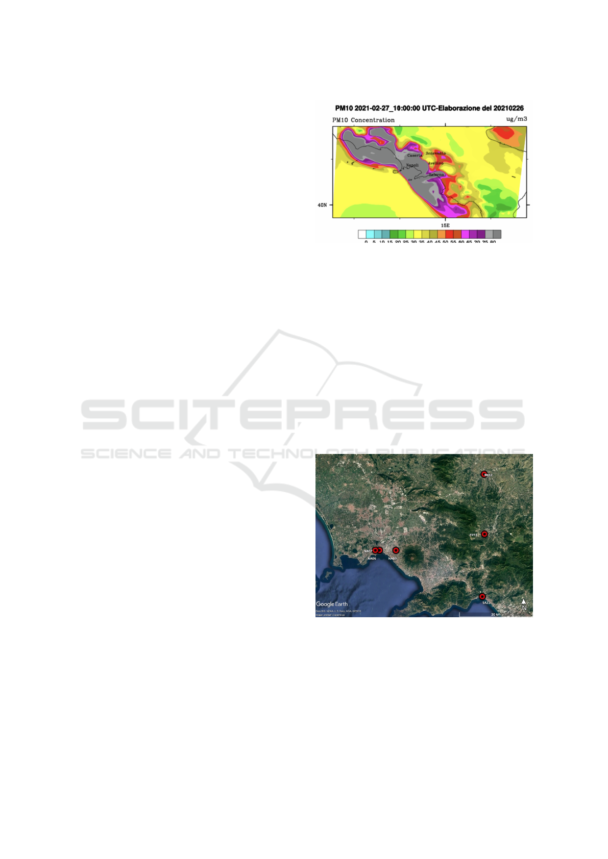
lutants concentration) cover a large area (Figure 1).

For this work, the ﬁrst check was made on the

open data regarding the concentration and the meteo-

rological speciﬁcs. The open data related to pollutants

concentration span since 2006 to 2018 (ARPAC, ),

while data about meteorological conditions are avail-

able since 2018 (Centro Meteorologico e Climato-

logico, ). In addition, not all the stations are able to

determinate the required pollutants: indeed, the sen-

sors need to be checked frequently, hence they can be

out of use for maintenance or, essentially, may be not

designed to cover all kinds of analyses.

The spatiotemporal discrepancy is analysed in or-

der to choose the boundary system. By matching the

Figure 1: Screenshot of the hourly forecasting of PM

made by ARPAC for February 26th, 2021. The area anal-

ysed was all the Campania region. The major cities are

identiﬁed with the black dots. In order to give a distance

set-up, it is highlighted that the distance Napoli - Caserta is

30 km circa. The prediction is calculated for three days.

two datasets, it is clear that the discrepancy is over-

come only since 2018 and only for those stations that

have recorded meteorological data. Figure 2 shows

the location of all the stations that provide both mete-

orological and concentration data and in Table 1 sta-

tions coordinates are reported.

We decided to work only on the stations in the city

of Napoli, so to restrict the area to be studies, aiming

at getting a better resolution for that speciﬁc city. The

chosen stations are reported in Table 2 with the spec-

iﬁcation of the pollutants analysed by each of them.

Figure 2: Satellite image of Napoli gulf (south-west), part

of Salerno gulf (south) and Piana Campana (north). The

red dots represent the locations of the stations with both

meteorological and concentration acquisition systems.

4 METHODOLOGY

One of the major concerns in any experiment which

tries to extract information from raw data, to obtain

Applying Machine Learning to Weather and Pollution Data Analysis for a Better Management of Local Areas: The Case of Napoli, Italy

357

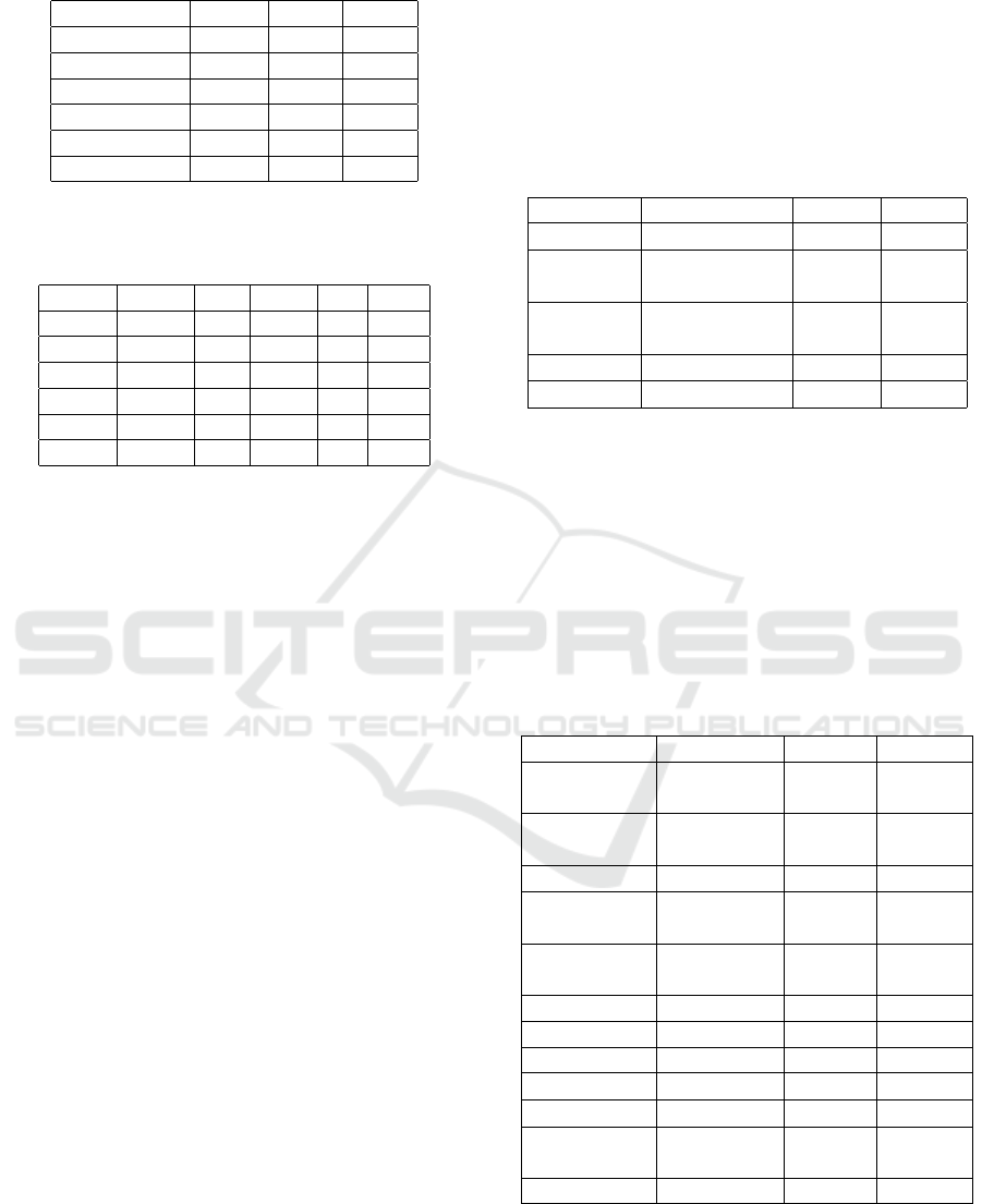
Table 1: Stations locations.

Station Code Name Long Lat

IT0898A NA06 14.25 40.85

IT0934A BN32 14.78 41.13

IT0936A AV41 14.78 40.91

IT1491A NA07 14.27 40.85

IT1493A NA09 14.35 40.85

IT1504A SA22 14.77 40.68

Table 2: Speciﬁc pollutants analysed by single station. T

stands for true, hence the contaminant is analysed. F stands

for false, so the contaminant is not analysed.

Name C

CO NO

NA06 T T T F F

BN32 F F T F F

AV41 T F T T F

NA07 T T T F T

NA09 T T T F F

SA22 F F T F F

hidden information and make predictions by machine

learning algorithms or other techniques, is the data

collection phase.

Data used in this experiment have been collected

by ARPAC ﬁxed stations located in the area managed

by Regione Campania; those data belong to two main

types of information: air pollution data and weather

data. Once acquired, those datasets should be merged

to have an unique dataset that includes all the values.

The resulting dataset is a good starting point for data

analysis and for applying regression models to obtain

predictions.

Besides the P.M., which is not revealed by these

stations, another important parameter to consider and

worth to predict is the CO: like the other compounds,

the carbon monoxide is used to classify the regional

area but, in contrast with the others, its average bench-

marks are calculated every 8 hours, hence the preci-

sion of the forecasting should be superior than that of

the forecasting of a pollutant with an average bench-

mark equal to 1 year.

4.1 Dataset Description

The air pollution dataset is downloaded from the of-

ﬁcial ARPAC website (ARPAC, ). The downloaded

dataset is in csv (comma separated values) format and

contains the entire acquired data volume. It is an ag-

gregate ﬁle that contains data from all sensors and all

stations collected hourly for year 2018.

The format used for the measurements in the csv

ﬁle is rather inconvenient for data analysis, as for each

sensor and station a different row is present. We have

transformed the dataset to obtain a ﬁle which has all

sensors value for each hour on the same line in order

to make the dataset more compact and manageable.

Parameters in the dataset are summarized in Ta-

ble 3: the relevant difference in the number of mea-

surements among the parameters depends on stations,

as stations only perform some measurements, like de-

scribed before.

Table 3: Parameters of air pollution dataset.

Parameter Description Unit n.

Benzene mg/m

29,205

CO Carbon mg/m

23,199

monoxide

Nitrogen mg/m

35,903

dioxide

Ozone mg/m

3,907

Sulfur dioxide mg/m

7,786

Weather data are downloaded from CEMEC web-

site. Differently from the previous case, in this one

a data ﬁle for each day must be downloaded. Each

ﬁle contains the measurements of a sensor and sta-

tion per line. Before applying the same transforma-

tion performed on the air pollution dataset, all ﬁles

have been merged in order to have an unique and con-

tinuous dataset.

Parameters in this dataset are summarized in Table

Table 4: Parameters of weather dataset.

Parameter Description Unit n.

AlbeInf Lower W /m

55,031

albedo

AlbeSup Upper W /m

55,031

albedo

Rainfall - mm 139,601

RadSG Day W /m

92,997

radiation

RadSN Night W/m

92,993

radiation

Temperature - C 155,250

Humidity - % 141,235

Pressure - hPa 134,735

UVA - W /m

55,507

UVB - W/m

55,529

Wind - degrees 70,149

direction

Wind speed - m/s 70,232

AI4EIoTs 2021 - Special Session on Artiﬁcial Intelligence for Emerging IoT Systems: Open Challenges and Novel Perspectives

358

4.2 Data Fusion

Once we had the raw data of both datasets available

in a manageable form, to maximize possible exploita-

tion the weather and the air pollution databases were

merged on same common information: the date and

time value of the measurement and the identiﬁer of

the station which measured them. This part is crucial

to preserve data correctness and to expand the useful

information content of the datasets.

Performing this transformation required coping

with the imbalance in the number of values avail-

able for the parameters in both datasets. To address

this issue we decided to utilize a maximum inclu-

sion strategy by performing the joining action with

”outer” mode to preserve the largest quantity of data

and avoid data loss.

If, on one hand, this procedure has allowed to ben-

eﬁt of all available data, on the other hand it has added

a new issue: the resulting dataset has a large num-

ber of missing elements caused by the missing values

for same parameters in the source datasets and am-

pliﬁed by the magnitude effect of Cartesian product

performed in the merging process.

4.3 Data Analysis

The data analysis of the new comprehensive dataset

has been executed mainly in Jupyter Notebook envi-

ronment using the Python programming language and

the Pandas library.

The ﬁrst step was oriented to obtain an insight into

the properties of each attribute of the dataset; the table

in ﬁgure 6 summarizes descriptive statistics of data.

As regression analysis could suffer bad perfor-

mances if there are highly correlated input features,

it is crucial to investigate the correlation between in-

put and output attributes. Consequently, in order to

guide a proper features selection, the second step ex-

plores the relationship between couples of variables:

the most common method for calculating this is Pear-

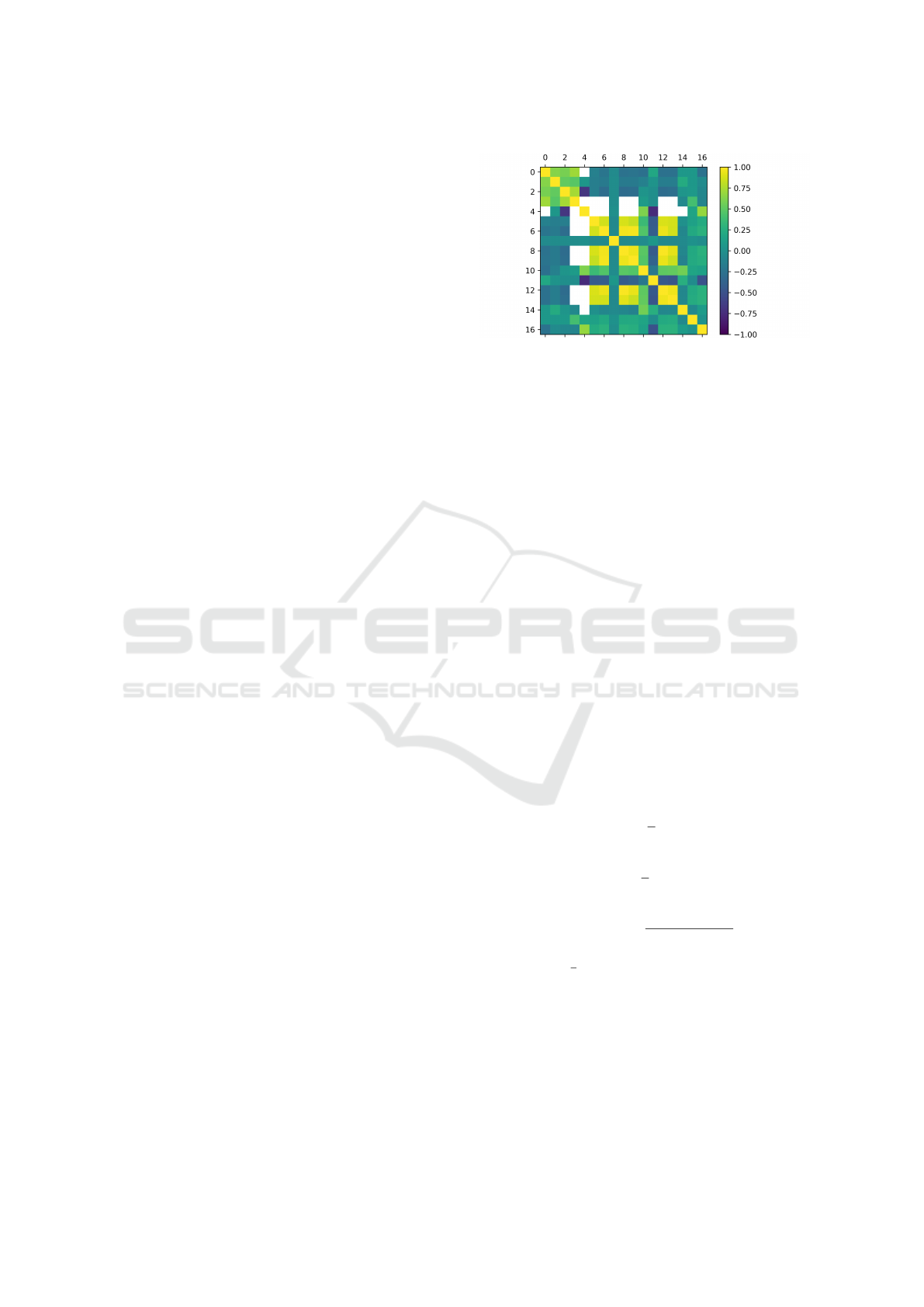
son’s Correlation Coefﬁcient. Figure 7 shows the cor-

relation matrix in which it can been seen the correla-

tion between all pairs of attributes. Figure 3 shows

the correlation matrix in graphical form.

Finally, a graphical analysis has been performed to

point out the characteristics of the attributes. Figure

4 and in Figure 5 provide a general outlook of the

distribution of each attributes.

The data analysis reveals some interesting facts

about the attributes. The AlbeInf, AlbeSup, RadSG,

RadSN, UVA and UVB have averagely high correla-

tion among them. It was widely expected, since they

measure different aspect of the solar radiation.

Figure 3: Correlation matrix plot.

In addition, the CO parameter has a moderate cor-

relation with C

, NO

and SO

, differently from all

the other attributes with which there is no evidence of

considerable correlation.

The last step in this phase consists in feature selec-

tion and data cleaning, therefore we drop some fea-

tures from the original dataset and drop all the lines

with missing data.

As ﬁnal result of data transformation, cleaning

and features selection, we have obtained a dataset

with the following features: C

, NO

, SO

, Rain-

fall, Temperature, Humidity, Pressure, Wind direc-

tion, Wind speed, and ﬁnally CO as target variable.

4.4 Evaluation Metrics

To validate the ability of the regression model to make

good predictions, the dataset has been divided into a

training and a test part, 70% and 30% respectively.

The Mean Square Error (MSE), the Mean Absolute

Error (MAE), and the Coefﬁcient of determination

) have been calculated to evaluate the performance

of prediction.

MAE(y, ˆy) =

n−1

∑

i=0

− ˆy

MSE(y, ˆy) =

n−1

∑

i=0

− ˆy

)

(y, ˆy) = 1 −

∑

i=1

− ˆy

)

∑

i=1

− ¯y)

where ¯y =

∑

i=1

MAE and MSE are risk metrics corresponding to

the expected value of the error and the quadratic error,

while R

(≤ 1) represents the proportion of variance

of y and provides a general indication of goodness of

ﬁt of the model.

Applying Machine Learning to Weather and Pollution Data Analysis for a Better Management of Local Areas: The Case of Napoli, Italy

359

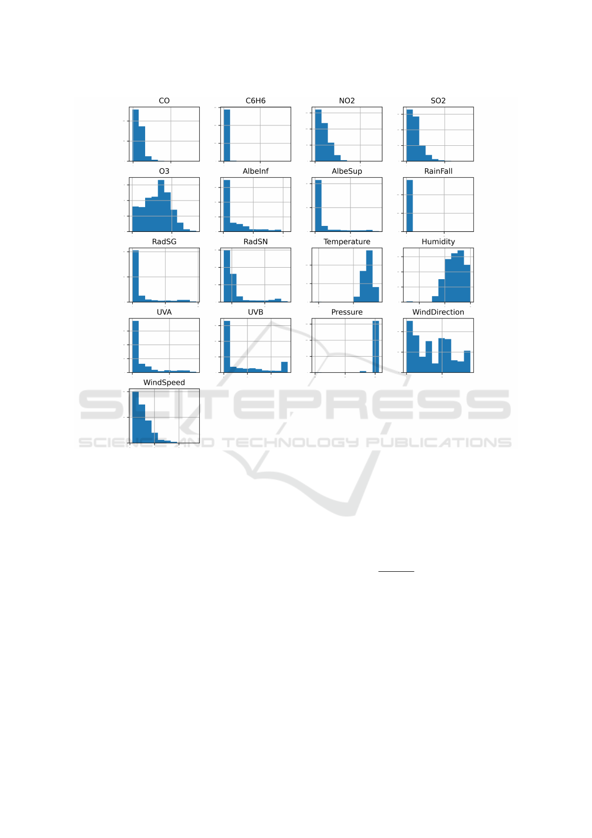
Figure 4: Outlook of distribution attributes.

4.5 Regression Models

In order to perform the analysis, we applied four dif-

ferent regression models, namely the Linear Regres-

sion Model calculated with Ordinary Least Square

(LN-OLS), the Ridge regression model (Ridge), the

Lasso model (Lasso) and Supervised Nearest Neigh-

bors Regression (KNN).

We use the notation x ∈ R

to describe the input

data, with m input features, y for the target variable

(CO). The Linear Model tries to approximate the pre-

dicted value ˆy using a linear combination of the input

features:

ˆy(w,x) = w

+ w

+ ... + w

We also use the notation X to describe the matrix

of input features and w = (w

,...,w

) for the vector

of coefﬁcients. Mathematically, the solution of the

following problem provides us with the values of the

coefﬁcients w of the linear model, using the afore-

mentioned methods:

OLS : min

kXw − yk

Ridge : min

kXw − yk

+ αkwk

Lasso : min

samples

kXw − yk

+ αkwk

The KNN was selected because it is a non linear

algorithm which uses a different approach, on a differ-

ent basis with respect to the other three chosen ones:

consequently, it is not possible to deﬁne an analogous,

yet consistent, formal expression.

5 RESULTS AND DISCUSSION

To implement the various regression algorithms, we

have used Python and the scikit-learn programming

AI4EIoTs 2021 - Special Session on Artiﬁcial Intelligence for Emerging IoT Systems: Open Challenges and Novel Perspectives

360

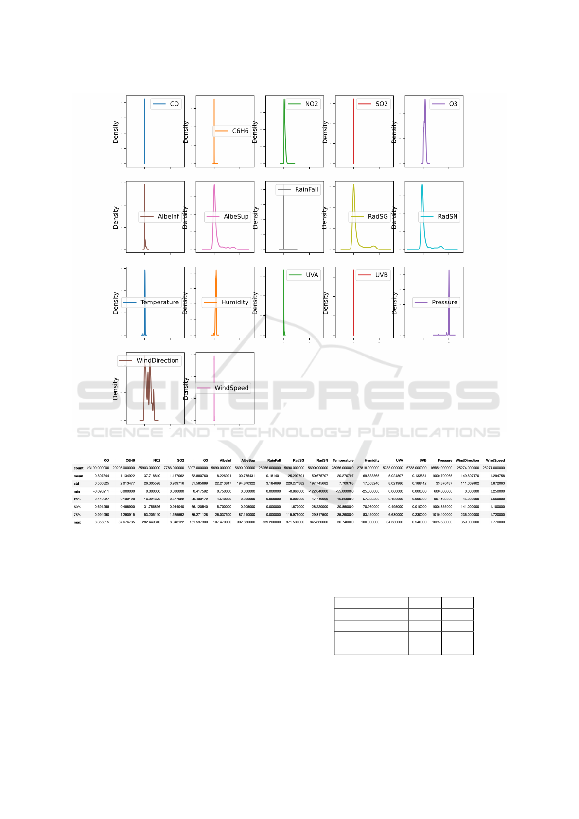
Figure 5: Outlook of attributes density.

Figure 6: Statistical outlook of attributes of the dataset.

library. We use a cross-validation approach, in or-

der to estimate the overall performance of the chosen

machine learning algorithms with less variance than

in the case of a single train-test split. The procedure

starts by dividing the dataset in k parts, with k = 10 in

our tests; then the algorithm is trained on k − 1 parts.

The result is a more reliable estimation of the perfor-

mance of the machine learning algorithm.

We have performed tests using variables X =

, NO

, SO

, Rainfall, Temperature, Humidity,

Pressure, Wind direction, Wind speed) as features and

variable y = CO as target. We have repeated tests for

each of the above considered machine learning algo-

rithms, obtaining comparable measurements of per-

formance. The results are summarised in Table 5.

Table 5: Results.

Model R2 MAE MSE

LR-OLS 0.73 0.12 0.04

Ridge 0.77 0.12 0.04

Lasso 0.60 0.13 0.05

KNN 0.68 0.12 0.04

This analysis intentionally uses only regression

models: the prediction of CO from weather measures

and other pollution-related values was not a straight-

Applying Machine Learning to Weather and Pollution Data Analysis for a Better Management of Local Areas: The Case of Napoli, Italy

361

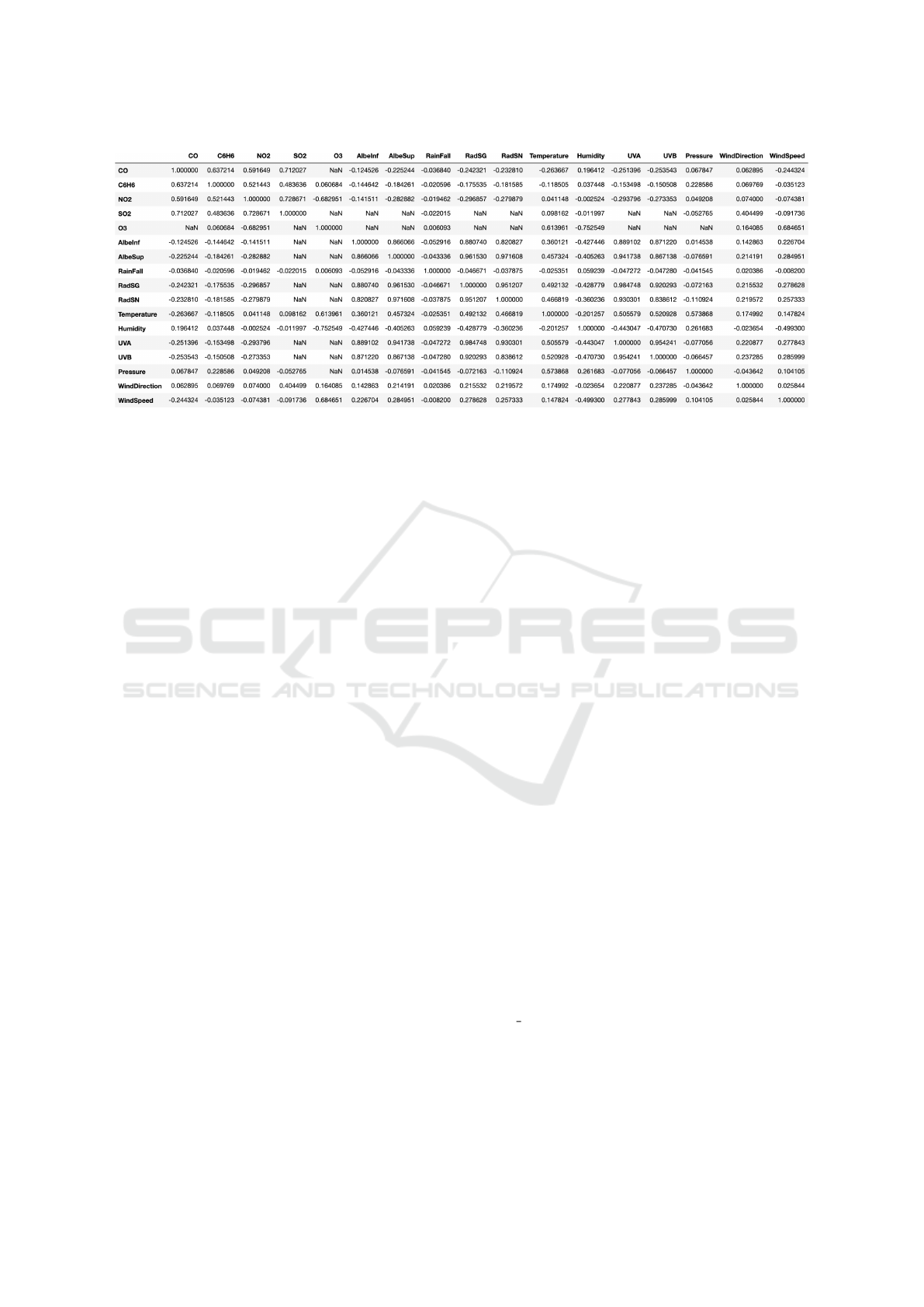
Figure 7: Pearson correlation between attributes of dataset.

forward task for the regression machine learning al-

gorithm, but with a R

value of 0.77 for the Ridge

algorithm and a low value for both MAE and MSE, it

becomes suitable for prediction.

6 CONCLUSIONS AND FUTURE

WORKS

In this paper we studied the applicability of a simple

machine learning technique on real open data man-

aged by third parties. Speciﬁcally, the analysed case

study is the Campania region (southern Italy), where

ARPAC, the local environmental protection agency,

developed and managed an air monitoring network by

using mobile and stationary stations. The same net-

work overlays with another network regarding mete-

orological measurements.

The ﬁrst step was the analysis of available data

and the creation of a merged dataset so to overcome

the spatiotemporal discrepancy. Indeed, even if the

same station can perform both the chemical analy-

sis and meteorological recording, the two networks

work on different layers; hence, data are recorded in

two different datasets with different characteristics.

The challenge was overcome with the use of identi-

ﬁers that linked the same station between the dataset

used. It is important to highlight that, other from

”outer” mode used to preserve the largest quantity of

data and avoid data loss, the data were not screened

for their coherence. This decision was made in or-

der to understand how coarse data perform with the

machine learning technique. According to the cor-

relation analysis performed on CO trends, this pa-

rameter emerged to have a moderate correlation with

, NO

and SO

, differently from all the other at-

tributes with which there is no evidence of consider-

able correlation. This correction is explained by the

characteristics of the compounds: all of them are re-

lated to vehicular trafﬁc emissions. Next, four differ-

ent regression models, namely the Linear Regression

Model calculated with Ordinary Least Square (LN-

OLS), the Ridge regression model (Ridge), the Lasso

model (Lasso) and Supervised Nearest Neighbors Re-

gression (KNN) were applied and evaluated by statis-

tical means. Finally, the Ridge regression model was

found to be the choice that ﬁts the best among them

with an R

value equal to 0.77 and low value for both

MAE and MSE, equal to 0.12 and 0.04 respectively.

In this work, using regression algorithms we only

scratched the surface in data prediction. The search

for a better prediction should consider the use of deep

learning algorithms: as a matter of fact, this method-

ology can analyse large datasets with considerable

performances. Nevertheless, it is clear that perform-

ing an headline validation of the starting data can help

both the techniques, as, at the moment, a human in-

tervention in the ﬁrst phases is still needed to address

the right directions in data exploration.

ACKNOWLEDGEMENTS

This work has been partially funded by the internal

competitive funding program “VALERE: VAnviteLli

pEr la RicErca” of Universit

a degli Studi della Cam-

pania “Luigi Vanvitelli” and by project ”Attrazione

e Mobilit

a dei Ricercatori” Italian PON Programme

(PON AIM 2018 num. AIM1878214-2).

AI4EIoTs 2021 - Special Session on Artiﬁcial Intelligence for Emerging IoT Systems: Open Challenges and Novel Perspectives

362

REFERENCES

Agarwal, S., Sharma, S., Suresh, R., Rahman, M. H.,

Vranckx, S., Maiheu, B., Blyth, L., Janssen, S., Gar-

gava, P., Shukla, V., et al. (2020). Air quality fore-

casting using artiﬁcial neural networks with real time

dynamic error correction in highly polluted regions.

Science of The Total Environment, 735:139454.

Armstrong, J. S. (2001). Extrapolation for Time-Series and

Cross-Sectional Data, pages 217–243. Springer US,

Boston, MA.

ARPAC. Organizzazione della rete di monitoraggio della

Qualit

a dell’Aria. https://dati.arpacampania.it/dataset/

rete-di-monitoraggio-della-qualita-dell-aria. Ac-

cessed: 2021-02-28.

Baklanov, A. and Zhang, Y. (2020). Advances in air quality

modeling and forecasting. Global Transitions, 2:261–

270.

Belavadi, S. V., Rajagopal, S., Ranjani, R., and Mohan, R.

(2020). Air quality forecasting using lstm rnn and

wireless sensor networks. Procedia Computer Sci-

ence, 170:241–248.

Brandt, J., Christensen, J. H., Frohn, L. M., Palmgren, F.,

Berkowicz, R., and Zlatev, Z. (2001). Operational air

pollution forecasts from european to local scale. At-

mospheric Environment, 35:S91–S98.

Campanile, L., Iacono, M., Lotito, R., and Mastroianni, M.

(2020). A wsn energy-aware approach for air pollu-

tion monitoring in waste treatment facility site: A case

study for landﬁll monitoring odour. In IoTBDS, pages

526–532.

Centro Meteorologico e Climatologico. http:

//cemec.arpa.campania.it/meteoambientecampania/

php/misure suolo.php. Accessed: 2021-02-28.

Chatﬁeld, C. (2000). Time-series forecasting. CRC press.

Contreras, L. and Ferri, C. (2016). Wind-sensitive interpo-

lation of urban air pollution forecasts. Procedia Com-

puter Science, 80:313–323.

Doma

nska, D. and Wojtylak, M. (2014). Explorative fore-

casting of air pollution. Atmospheric Environment,

92:19–30.

European Environmental Agency. European Air Qual-

ity Index. https://www.eea.europa.eu/themes/air/

air-quality-index. Accessed: 2021-02-28.

Haehnel, P., Mare

cek, J., Monteil, J., and O’Donncha, F.

(2020). Using deep learning to extend the range of

air pollution monitoring and forecasting. Journal of

Computational Physics, 408:109278.

Hyndman, R. J. and Athanasopoulos, G. (2018). Forecast-

ing: principles and practice. OTexts.

Kurt, A., Gulbagci, B., Karaca, F., and Alagha, O. (2008).

An online air pollution forecasting system using neu-

ral networks. Environment international, 34(5):592–

598.

Liu, H., Yan, G., Duan, Z., and Chen, C. (2021). Intelligent

modeling strategies for forecasting air quality time se-

ries: A review. Applied Soft Computing, page 106957.

Masmoudi, S., Elghazel, H., Taieb, D., Yazar, O., and

Kallel, A. (2020). A machine-learning framework for

predicting multiple air pollutants’ concentrations via

multi-target regression and feature selection. Science

of the Total Environment, 715:136991.

Masood, A. and Ahmad, K. (2020). A model for particu-

late matter (pm2. 5) prediction for delhi based on ma-

chine learning approaches. Procedia Computer Sci-

ence, 167:2101–2110.

Shetty, C., Sowmya, B., Seema, S., and Srinivasa, K.

(2020). Air pollution control model using machine

learning and iot techniques. In Advances in Comput-

ers, volume 117, pages 187–218. Elsevier.

Tong, W. (2020). Machine learning for spatiotemporal big

data in air pollution. In Spatiotemporal Analysis of Air

Pollution and Its Application in Public Health, pages

107–134. Elsevier.

Xiao, D., Fang, F., Zheng, J., Pain, C., and Navon, I. (2019).

Machine learning-based rapid response tools for re-

gional air pollution modelling. Atmospheric environ-

ment, 199:463–473.

Zhou, Y., Chang, F.-J., Chang, L.-C., Kao, I.-F., and Wang,

Y.-S. (2019). Explore a deep learning multi-output

neural network for regional multi-step-ahead air qual-

ity forecasts. Journal of cleaner production, 209:134–

145.

Applying Machine Learning to Weather and Pollution Data Analysis for a Better Management of Local Areas: The Case of Napoli, Italy

363