
The Estimation of Traffic Flow Parameters based on Monitoring the
Speed Values using Computer Vision
V. D. Shepelev
1a
, A. I. Vorobyev
2b
, E. V. Shepeleva
1c
, I. D. Alferova
1d
, N. Golenyaev
1e
,
G. Yakupova
3f
and V. G. Mavrin
3g
1
South Ural State University, 76 Lenin Prospekt, Chelyabinsk, Russia
2
Moscow Automobile and Road Construction State Technical University, 64, Leningradsky Prospect, Moscow, Russia
3
Kazan Federal University, 18 Kremlyovskaya str, Kazan, Russia
vadim_mmite@rambler.ru
Keywords: Monitoring, Neural Networks, Statistical Analysis, Traffic Capacity, Vehicle Speed, YOLOv3.
Abstract: Most of the previous works dealing with road traffic organization have been focused on optimizing the
setup of traffic signals, assuming that the traffic flow speed is fixed or adheres to a given distribution. In our
study, we focused on real-time determining the vehicle speed and assessing its influence on the vehicle
delay time. Vehicle detection and speed determination are based on real-time processing of video streams
by a convolutional neural network (YOLOv3). The developed system can identify and classify traffic flows
into eleven types, as well as track the motion path and speed of vehicles throughout the entire functional
area of a signal-controlled intersection. While analysing the data, we identified two important factors
corresponding to the presence of a queue of vehicles waiting for the green traffic light: 1. We identified the
nature and statistically significant measure of reducing the free vehicle movement speed, depending on the
size of the queue; 2. We determined the acceptable queue size, which does not affect the dynamics of
crossing the intersection by group vehicles moving from the previous intersection. The obtained data allows
us to optimize the operation of the adaptive traffic light control of intersections and to optimize the
synchronization of road network signals based on speed indications.
a
https://orcid.org/0000-0002-1143-2031
b
https://orcid.org/0000-0002-1890-6033
c
https://orcid.org/0000-0003-2080-3145
d
https://orcid.org/0000-0001-8484-8129
e
https://orcid.org/0000-0003-3657-3567
f
https://orcid.org/0000-0001-6822-3700
g
https://orcid.org/0000-0001-6681-5489
1 INTRODUCTION
Most of the previous studies on the optimization of
road traffic parameters (Wong et al., 2010; Wong
et al., 2011), including methods for the
synchronization of coordinated signals
(Skabardonis and Geroliminis, 2008; Liu et al.,
2011; Makarova et al., 2020) are focused on the
optimization of signal timings ignoring the speed
of traffic flows (Wu et al., 2015; Makarova et al.,
2017). The real-time movement speed depends on
several factors, including the condition and quality
of the road surface, the driver behaviour, the
vehicle performance characteristics, and road
conditions (Burkhardt et al., 2021; Tian et al.,
2021). Variable speed can be used on highways to
control the traffic flow to increase the traffic
capacity in open highway sections. In particular,
the procedure for detecting road accidents is
considered in (Allaby et al., 2007; Hadiuzzaman et
al., 2013; Škorput et al., 2010; Beymer et al.,
1997). In the studies focused on monitoring the
level of traffic flow emissions, the key input
variables are instantaneous measurements of the
752
Shepelev, V., Vorobyev, A., Shepeleva, E., Alferova, I., Golenyaev, N., Yakupova, G. and Mavrin, V.
The Estimation of Traffic Flow Parameters based on Monitoring the Speed Values using Computer Vision.
DOI: 10.5220/0010539407520759
In Proceedings of the 7th International Conference on Vehicle Technology and Intelligent Transport Systems (VEHITS 2021), pages 752-759
ISBN: 978-989-758-513-5
Copyright
c
2021 by SCITEPRESS – Science and Technology Publications, Lda. All rights reserved

vehicle speed and acceleration (Ahn et al., 2002;
Pavlovic et al., 2021). Therefore, it is essential to
closely monitor the flow speed, which can facilitate
making effective management decisions, as well as
predicting the influence of vehicle emissions on the
ambient air quality (Agarwal and Mustafi, 2021).
There are methods for detecting anomalies and
interpreting road traffic analysis using the Global
Navigation Satellite System (GNSS). The method
is based on measuring the Euclidean distance
between the STM (Speed Transition Matrices)
centre of mass (COM) and the mean STM, which
represents normal driving conditions. Space and
time-related events are combined into so-called
traffic congestion propagation patterns. These
patterns provide a high-level description of traffic
congestion and its propagation in time and space
(Tisljaric et al., 2020; Wang et al., 2013). This
approach is characterized by a significant data
transmission delay and averaging, which does not
allow one to instantly receive and respond to any
deviations in traffic parameters.
The vehicle speed determines the time the
vehicle needs to cross the functional area of the
intersection. The authors of (Wang, 2007)
considered a general approach to the development
of universal means for assessing the state of road
traffic for highway sections based on stochastic
macroscopic traffic modelling and extended
Kalman filtering. Vakili et al. (2020), Czajewski
and Iwanowski (2010) present a speed calculation
method based on the use of geometric information
and the distance travelled by vehicles. The
algorithms are based on processing a video image
taken by a single camera on the road to extract the
license plate in the image.
In this study, we focused on developing a
method for traffic speed monitoring to determine
the delay time of the vehicle queue. The main
objectives of this paper are: 1) to highlight the
nature and statistically significant measure of
reducing the free vehicle movement speed in the
presence of a queue in front of a traffic light; 2) to
determine the size of the queue, which does not
affect the dynamics of crossing the intersection by
group vehicles.
Although speed is very important to ensure the
safety and efficiency of setting road traffic control
systems (Choi et al., 2013; Makarova et al., 2018),
and there are known advantages of integrating
speed into traffic signal synchronization programs
(Abu-Lebdeh, 2010; Daganzo and Pilachowski,
2011), there remain technical difficulties in a
reliable real-time determination of the driving
speed and interpretation of big data.
2 DEVELOPMENT OF A
METHOD OF DETERMINING
THE VEHICLE SPEED
Our approach is based on the use of street video
surveillance cameras with a viewing angle
providing visibility of the entire functional area of
the intersection and the adjacent roads (Online
broadcast). We used the architecture of the
YOLOv3 neural network, which consists of 106
layers and is a modification of the Darknet-53
neural network (Khazukov et al., 2020). Besides, it
includes 53 more layers with two N-dimensional
output layers providing for the detection at three
different scales. This modification contributes to
more accurate vehicle recognition and
classification. As input data, YOLOv3 accepts an
image represented as a three-dimensional tensor
h×w×3, where h, w is the height and length of the
input image. We used OpenCV open-source library
to work with machine vision algorithms and
process images and general-purpose numerical
algorithms. To track traffic flows, we used the Sort
library built on elementary data associations and
methods for assessing the state of objects. To
calculate the vehicle speed, we need to find the
distance travelled based on the change in the
latitude and longitude of the object location, using
the change in coordinates. To solve this problem,
we calculated the perspective transformation matrix
(1) by selecting reference points in the map and
comparing their corresponding points in the image
(Figures 1, 2) (Khazukov et al., 2020).
Figure 1: Reference points in the image.
The Estimation of Traffic Flow Parameters based on Monitoring the Speed Values using Computer Vision
753
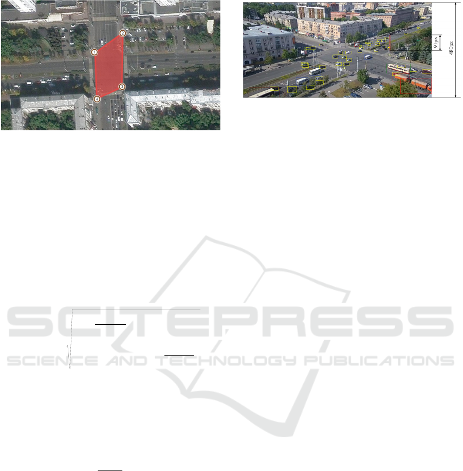
Figure 2: Reference points in the image.
′
′
=
×
i
i
i
i
i
t
y
x
y
x
A
1
(1)
where A is the perspective transformation matrix, x
i
,
y
i
are the pixel coordinates in the image; x´
i
, y´
i
are
the latitude and longitude of a point in the image.
We will calculate the distance between two
points based on the formula of inverse haversine
presented explicitly through the arcsine:
() ()
−
+
+
−
⋅=
2
sincoscos
2
sin
arcsin2
12
2
12
12
2
λλ
ϕϕ
ϕϕ
rD
(
2)
where D is the measured distance; φ
i
, λ
i
are the
latitude and longitude of the i-th point; r =6.371 km
is the earth radius.
We will find the average speed by the following
formula:
12
tt
D
v
−
=
(3)
where t
1
, t
2
is the time of the beginning and the end
of the object movement at a distance.
The distance measurement accuracy is calculated
and verified based on a perspective transformation
determining the area of the used pixels transmitting
the road section (Figure 3).
The actual size of the marked distance is 88.5 m,
in the image this segment is transmitted as 91px.
One pixel in this section covers an area with a
length of 0.97 m. Taking this area as a square, we
Figure 3: The distance transmitted by pixels.
can estimate the maximum projection error of a
point within this area of 1.37 m. Thus, the error in
determining the speed does not exceed 1.7 km/h.
2.1 Statistical Significance of
Differences
In statistical analysis, it is generally accepted to
consider the revealed regularity to be statistically
significant when the empirical level of significance
is less than the generally accepted critical value of
0.05 (5%) (Byul, 2005; Tyurin and Makarov, 2016).
For the considered problem of estimating the
statistical significance of reducing the time spent on
crossing the intersection in the presence of a queue,
we should make sure that the calculated mean values
of time (Table 1), from the standpoint of statistics,
are not in the same confidence interval, i.e., they do
not represent the same numeric value.
We used the professional SPSS Statistical
Analysis Package for the calculations. According to
Table 1, the empirical significance levels of
deviations are much lower than the limiting ones,
which indicates the statistical significance of the
vehicle speed deviations in the presence of a queue
before the intersection.
The SPSS package additionally calculates paired
Pearson correlation coefficients between the same
variables (Table 2), which show a weak correlation
between them.
This additionally confirms the legitimacy of the
conclusion that the changes in the vehicle speeds are
statistically significant - due to the absence of
hidden regularities in empirical data, which could
distort the analysis results.
The recommended verification of the results of
the statistical significance of the differences in the
speed of the vehicles passing the intersection in the
interpretation of the nonparametric approach also
confirmed the high significance of its change. Table
3 presents the results of the calculations using the
Wilcoxon nonparametric signed-rank test.
iMLTrans 2021 - Special Session on Intelligent Mobility, Logistics and Transport
754

Table 1: Statistical significance of the deviations of the intersection crossing speeds.
Paired differences t Degrees
of
freedom
Significance
Mean Standard
deviation
Pair 1 Och1 & OchN 1.43704 1.33611 12.497 134 0.00
Pair 2 Och1 & NoOch1 2.02133 1.403367 16.732 134 0.00
Pair 3 Och1 & NoOchN 3.00489 1.37474 25.397 134 0.00
Pair 4 OchN & NoOch1 0.58430 1.11680 6.079 134 0.00
Pair 5 OchN & NoOchN 1.56785 0.96799 18.819 134 0.00
Pair 6 NoOch1 & NoOchN 0.98356 1.10166 10.373 134 0.00
Table 2: Correlation of paired samples.
N Correlation Significance
Pair 1 Och1 & OchN 135 0.230 0.007
Pair 2 Och1 & NoOch1 135 0.199 0.020
Pair 3 Och1 & NoOchN 135 0.067 0.438
Pair 4 OchN & NoOch1 135 0.284 0.001
Pair 5 OchN & NoOchN 135 0.286 0.001
Pair 6 NoOch1 & NoOchN 135 0.177 0.041
Table 3: Statistical significance by the Wilcoxon test.
Z
Asymptotic
significance
(two-sided)
OchN - Och1 -8.584
a
0.00
NoOch1 - Och1 -9.456
a
0.00
NoOchN - Och1 -10.048
a
0.00
NoOch1 - OchN -5.515
a
0.00
NoOchN - OchN -9.644
a
0.00
NoOchN - NoOch1 -7.666
a
0.00
2.2 Analysis of the Vehicle Queue Size
This study is based on the video camera data on the
operation of 22 urban intersections and, similarly,
assumes the solution of the following tasks:
1. additional processing of the initial data to
make them homogeneous;
2. analysis of the mean values of the intervals
between the vehicles located in different
initial positions in the queue in front of a
traffic light when they enter the intersection;
3. determination of the queue size, when the last
vehicle in the queue passes the intersection as
if there is no delay in the queue.
2.2.1 Formation of a Homogeneous Sample
The previous clustering of the analysed intersections
showed a contrast in the empirical data for the two
intersections containing tram lines. Therefore, for
further analysis, we use about 30 observations for
each of the twenty intersections quite similar in the
way they are passed by vehicles. Eventually, for the
analysis in this task, we used 590 records of passing
the vehicle queue only on the green traffic light.
Similar to the first study, we removed the
observations for the transport categories other than
M1 (vehicles, which are used to carry passengers
and have no more than eight seats in addition to the
driver’s seat), M2 (vehicles, which are used to carry
passengers, have more than eight seats in addition to
the driver’s seat, the technically permissible
maximum mass of which does not exceed <5 t), and
N1 (small trucks with the technically permissible
maximum mass not exceeding <3.5 t.) from the
empirical data (Classification of vehicles according
to technical regulations, 2018). The size of the
vehicle queue considered in this study is limited by
the availability of a sufficient amount of the
empirical data – these are 13 vehicles. According to
the final results, it turned out to be sufficient to form
reliable conclusions.
The Estimation of Traffic Flow Parameters based on Monitoring the Speed Values using Computer Vision
755
2.2.2 Mean Values of the Time Needed to
Pass the Intersections by the Vehicle
Queue
The summary calculated data on processing the
sample of observations of passing twenty
intersections by a vehicle queue are presented in
summary Table 4.
Notably, the table clearly shows the difference
between the intersections in the dynamics of
crossing by vehicles. This has been shown earlier
when the intersections were clustered into
homogeneous groups. However, in this task, this
difference does not affect the distortion of the
general trend but only emphasizes the generality of
the conclusions obtained for various intersections.
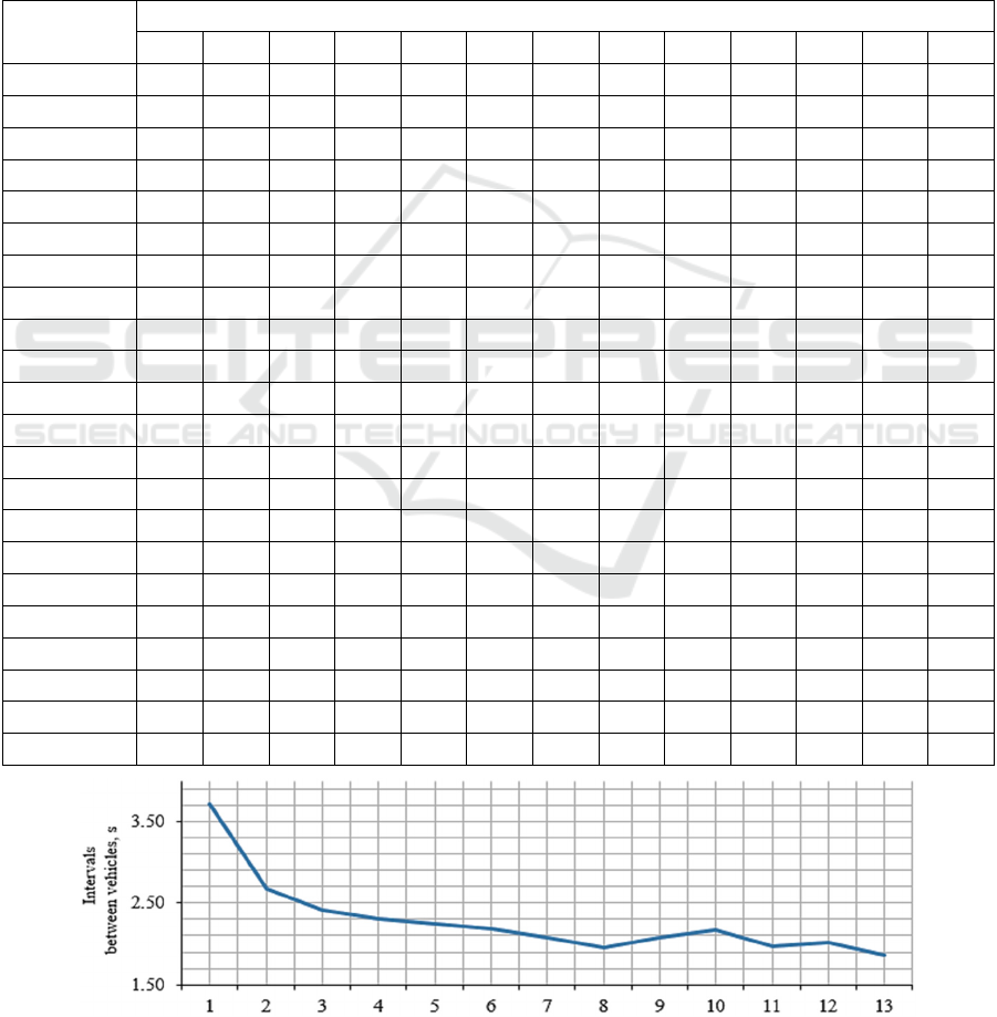
The processing results are graphically shown in
Figure 4, where the horizontal axis indicates the
position of the vehicle in the queue before the
intersection, and the vertical axis indicates the mean
time of the interval this vehicle needs to enter the
intersection.
Table 4: Mean time of the intervals the vehicles need to enter the intersection.
Intersections
Position of the vehicle in the queue
1 2 3 4 5 6 7 8 9 10 11 12 13
Prkr01 3.0 2.9 2.7 2.3 2.6 2.5 2.4 1.8 2.2 2.3 2.8 2.0 2.0
Prkr02 3.5 3.6 2.5 3.1 2.7 2.3 2.1 2.1 2.0 2.1 2.0 2.0 1.5
Prkr03 3.4 2.8 2.7 2.4 2.2 2.3 2.4 2.0 2.5 2.0 1.9 1.6 1.6
Prkr04 3.0 3.0 2.7 2.1 2.4 1.5
Prkr05 2.6 2.8 2.2 1.7 2.4 1.8 2.0 1.5 1.5 2.0
Prkr06 3.0 2.8 2.3 2.5 2.0 2.0 2.2 1.6 2.0
Prkr07 4.2 2.3 2.1 2.1 2.0 2.0 1.8 2.2 1.6
Prkr08 3.4 3.5 2.8 2.8 3.0 2.0 2.4 2.7 2.3 2.5
Prkr09 4.5 2.8 2.7 2.1 2.0 2.0
Prkr10 4.1 2.2 1.9 1.8 2.1 2.1 2.0 1.6 2.0 2.0 2.4 2.2 1.8
Prkr11 3.1 2.4 2.2 2.0 1.9 2.0 2.0 1.8 1.7 2.6 1.7 2.0 2.2
Prkr12 2.9 2.5 2.5 2.5 2.0 2.4 1.9 1.8 2.2 2.1 2.5 2.2 1.7
Prkr13 3.0 2.8 2.3 2.7 1.5 2.0
Prkr14 3.0 2.6 2.4 2.3 2.6 3.0 2.0 2.0 2.0
Prkr15 4.6 2.2 2.3 2.3 2.2 2.0
Prkr16 5.1 2.1 2.0 2.0 2.0 2.0
Prkr17 4.6 2.8 2.5 2.7 2.5 3.0 2.0
Prkr18 3.7 2.6 2.8 2.4 2.1 2.8 2,2 2.2 2.9 1.8 1.5 2.0 2.0
Prkr19 3.8 1.9 1.9 1.7 2.0 1.8 1.6 1.7 1.6 2.6 1.3 2.0
Prkr20 5.2 2.2 1.9 2.0 2.1 1.8 1.7 1.8 2.2 1.5 1.5
Mean: Sr1 Sr2 Sr3 Sr4 Sr5 Sr6 Sr7 Sr8 Sr9 Sr10 Sr11 Sr12 Sr13
3.72 2.69 2.41 2.31 2.24 2.19 2.07 1.96 2.08 2.16 1.97 2.01 1.86
Figure 4: The intervals a vehicle needs to enter the intersection, depending on its position in the queue.
iMLTrans 2021 - Special Session on Intelligent Mobility, Logistics and Transport
756

We can assume a priori that the dynamics of the
vehicles passing the intersection, starting from the
7th vehicle in the queue, becomes stable.
That is, a queue of six vehicles or more already
does not slow down the time of passing the
intersection by subsequent vehicles. The mean time
of the interval between vehicles entering the
intersection is two seconds.
However, these preliminary conclusions should
be confirmed in terms of their statistical
significance.
2.2.3 The Size of the Queue Stabilizing the
Interval between Vehicles
Taking into account the significant influence of the
human factor in fixing empirical data, as well as
their major gradation by an observer within one
second, a nonparametric approach used in similar
conditions will be more suitable for statistical
analysis. Moreover, the normal distribution of the
initial data is out of the question.
Notably, the samples are linked through the
observed intersections. Therefore, the statistical
analysis method most suitable in this study is the
Wilcoxon nonparametric signed-rank test for two
linked samples (SPSS statistical analysis package).
We will use this method to check the possible pairs
of differences of all the calculated mean values of
the Sr1-Sr13 intervals from the a priori assumed
SR0 value of two seconds.
The calculation results are presented in Table 5.
According to the calculations, the mean values,
starting from Sr6, fall into the confidence interval of
the a priori expected value of two seconds, i.e., they
Table 5: Statistical significance by the Wilcoxon test.
Z
Asymptotic
significance
(two-sided)
SR0-Sr1 -3.922
a
0%
SR0-Sr2 -3.885
a
0%
SR0-Sr3 -3.696
a
0%
SR0-Sr4 -2.940
a
0.3%
SR0-Sr5 -2.728
a
0.6%
SR0-Sr6 -1.790
a
7.4%
SR0-Sr7 -1.716
a
8.6%
SR0-Sr8 -1.171
b
24.2%
a. Positive ranks are used
b. Negative ranks are used
become statistically indistinguishable. This means
that in the queue before the intersection, vehicles,
starting from the 6th position in the queue, pass the
intersection with the time intervals corresponding to
the absence of a queue. This time interval
corresponds to the generally accepted estimates of
two seconds.
Notably, the mean values of the intervals
corresponding to the vehicles’ positions from 9 to 13
are not considered due to the decreasing amount of
the initial data and because their absolute values are
much closer to the a priori expected SR0 value than
for SR6.
3 CONCLUSIONS
In the course of the study, we identified two
important factors corresponding to the presence of a
vehicle queue before the intersection on the red
traffic light.
First, we revealed the nature and statistically
significant measure of reducing the free movement
vehicle speed in the presence of a queue in front of
the traffic light.
Second, we determined the size of the queue,
which does not affect the dynamics of passing the
intersection by the vehicles following the queue. We
also determined their mean interval of movement
equal to two seconds.
In addition to these two factors manifested and
studied in this paper, which correspond to the
presence of a vehicle queue, we can note other
interesting areas of research, such as a
heterogeneous structure of the category of vehicles
in the queue, their location in the queue, and several
other important situations. These areas are the
subject of our further research generally intended for
task-oriented vehicle flow management.
REFERENCES
Abu-Lebdeh, G., 2010. Exploring the potential benefits of
IntelliDrive-enabled dynamic speed control in
signalized networks. Proceedings of the 89th Annual
Meeting of the Transportation Research Board, # 10-
3031.
Agarwal, A.K., Mustafi, N.N., 2021. Real-world
automotive emissions: Monitoring methodologies, and
control measures. Renewable and Sustainable Energy
Reviews, 137(110624).
Ahn, K., Rakha, H., Trani, A., Van Aerde, M., 2002.
Estimating vehicle fuel consumption and emissions
based on instantaneous speed and acceleration levels.
The Estimation of Traffic Flow Parameters based on Monitoring the Speed Values using Computer Vision
757

Journal of Transportation Engineering, 128 (2): 182-
190.
Allaby, P., Hellinga, B., Bullock, M., 2007. Variable
speed limits: Safety and operational impacts of a
candidate control strategy for freeway applications.
IEEE Transactions on Intelligent Transportation
Systems, 8 (4): 671-680.
Atev, S., Masoud, O., Janardan, R., Papanikolopoulos, N.,
2005. A collision prediction system for traffic
intersections. In Proceedings of the IEEE/RSJ
International Conference on Intelligent Robots and
Systems (IROS), 1545407: 169-174.
Beymer, D., McLauchlan, P., Coifman, B., Malik, J.,
1997. Real-time computer vision system for measuring
traffic parameters. In Proceedings of the IEEE
Computer Society Conference on Computer Vision
and Pattern Recognition, pp. 495-501.
Buch, N., Cracknell, M., Orwell, J., Velastin, S.A., 2009.
Vehicle localisation and classification in urban CCTV
Streams. In Proceedings of the 16th World Congress
on Intelligent Transport Systems and Services (ITS
2009)
Buch, N., Velastin, S.A., Orwell, J., 2011.A review of
computer vision techniques for the analysis of urban
traffic. IEEE Transactions on Intelligent
Transportation Systems, 12 (3) # 5734852: 920.
Buch, N., Yin, F., Orwell, J., Makris, D., Velastin, S.A.,
2009. Urban vehicle tracking using a combined 3D
model detector and classifier. Lecture Notes in
Computer Science, 5711 LNAI (PART 1): 169-176.
Buivol, P.A., Iakupova, G.A., Makarova, I.V.,
Mukhametdinov, E.M., 2020. Search and optimization
of factors to improve road safety. International Journal
of Engineering Research and Technology, 13
(11):3751-3756.
Burkhardt, M., Yu, H., Krstic, M., 2021. Stop-and-go
suppression in two-class congested traffic.
Automatica, 125(109381).
Byul, A., 2005. SPSS: the art of information processing.
Statistical data analysis and recovery of hidden
patterns. Moscow, DiaSoft.
Choi, J., Tay, R., Kim, S., 2013. Effects of changing
highway design speed. Journal of Advanced
Transportation, 47(2): 239-246.
Classification of vehicles according to technical
regulations (November 2018). Available at https://xn--
80aaf3axmme8h.xn--p1ai/registratsiya-i-uchet/klassifi
katsiya-ts
Czajewski, W., Iwanowski, M., 2010. Vision-based
vehicle speed measurement method. Lecture Notes in
Computer Science, 6374 LNCS (PART 1): 308-315.
Dailey, D.J., Cathey, F.W., Pumrin, S., 2000.An algorithm
to estimate mean traffic speed using uncalibrated
cameras. IEEE Transactions on Intelligent
Transportation Systems, 1 (2): 98-107.
Gunawan, A.A.S., Tanjung, D.A., Gunawan, F.E., 2019.
Detection of vehicle position and speed using camera
calibration and image projection methods. Procedia
Computer Science, 157: 255-265.
Hadiuzzaman, M., Qiu, T.Z., 2013. Cell transmission
model based variable speed limit control for freeways.
Canadian Journal of Civil Engineering, 40 (1): 46-56.
Khazukov, K., Shepelev, V., Karpeta, T., Shabiev, S.,
Slobodin, I., Charbadze, I., Alferova, I., 2020. Real-
time monitoring of traffic parameters. Journal of Big
Data, 7 (1), # 84.
Kim, H., 2019. Vehicle detection and speed estimation for
automated traffic surveillance systems at nighttime.
Tehnicki Vjesnik, 26 (1): 87-94.
Maduro, C., Batista, K., Batista, J., 2009. Estimating
vehicle velocity using image profiles on rectified
images. Lecture Notes in Computer Science, 5524
LNCS: 64-71.
Makarova, I., Pashkevich, A., Shubenkova, K., 2017.
Ensuring Sustainability of Public Transport System
through Rational Management. In Proceedings of the
16th International Scientific Conference Reliability
and Statistics in Transportation and Communication,
178: 137-146.
Makarova, I., Shubenkova, K., Mavrin, V., Buyvol, P.,
2018. Improving safety on the crosswalks with the
use of fuzzy logic, Transport Problems, 13 (1): 97-
109.
Makarova, I., Yakupova, G., Buyvol, P., Mukhametdinov,
E., Pashkevich, A., 2020. Association rules to identify
factors affecting risk and severity of road accidents. In
Proceedings of the 6th International Conference on
Vehicle Technology and Intelligent Transport Systems
(VEHITS), 614-621.
Online broadcast. Video surveillance. 2021. Availible at
https://cams.is74.ru/live
Pavlovic, J., Fontaras, G., Broekaert, S., Ciuffo, B.,
Ktistakis, M.A., Grigoratos, T., 2021. How accurately
can we measure vehicle fuel consumption in real
world operation? Transportation Research Part D:
Transport and Environment, 90(102666).
Škorput, P., Mandžuka, S., Jelušić, N., 2010. Real-time
detection of road traffic incidents. Promet - Traffic -
Traffico, 22 (4): 273-283.
Tian, J., Zhu, C., Chen, D., Jiang, R., Wang, G., Gao, Z.,
2021. Car following behavioural stochasticity analysis
and modeling: Perspective from wave travel time.
Transportation Research Part B: Methodological,
143:160-176.
Tisljaric, L., Majstorovic, Z., Erdelic, T., Caric, T., 2020.
Measure for traffic anomaly detection on the urban
roads using speed transition matrices. In Proceedings
of the 43rd International Convention on Information,
Communication and Electronic Technology (MIPRO),
9245327: 252-259.
Tyurin, Yu. N., Makarov, A. A., 2016. Data analysis on a
computer: textbook. Moscow, ICNMO.
Vakili, E., Shoaran, M., Sarmadi, M.R., 2020. Single–
camera vehicle speed measurement using the geometry
of the imaging system. Multimedia Tools and
Applications, 79 (27-28): 19307-19327.
Wang, Y., Papageorgiou, M., Messmer, A., 2007. Real-
time freeway traffic state estimation based on
iMLTrans 2021 - Special Session on Intelligent Mobility, Logistics and Transport
758

extended Kalman filter: A case study. Transportation
Science, 41 (2): 167-181.
Wang, Z., Lu, M., Yuan, X., Zhang, J., Wetering, H.V.D.,
2013. Visual traffic jam analysis based on trajectory
data. IEEE Transactions on Visualization and
Computer Graphics, 19 (12), 6634174: 2159-2168.
Wu, W., Li, P.K., Zhang, Y., 2015. Modelling and
simulation of vehicle speed guidance in connected
vehicle environment. International Journal of
Simulation Modelling, 14 (1): 145-157.
Young, C., Rice, J., 2006. Estimating velocity fields on a
freeway from low-resolution videos. IEEE
Transactions on Intelligent Transportation Systems, 7
(4): 463-469.
The Estimation of Traffic Flow Parameters based on Monitoring the Speed Values using Computer Vision
759
