Property Lifecycle Diagram for Tracing State Machine Diagram Changes

Shinpei Ogata

1 a

, Yusuke Nishizawa

, Erina Makihara

2 b

, Mizue Kayama

1 c

and Kozo Okano

Faculty of Engineering, Shinshu University, 4–17–1 Wakasato, Nagano, Japan

Faculty of Science and Engineering, Doshisha University, 1–3 Tatara Miyakodani, Kyoto, Japan

Keywords:

Edit Log, Modeling Process, State Machine Diagram, Visualization.

Abstract:

For geographically distributed systems such as IoT (Internet of Things) and CPS (Cyber-Physical System),

those systems provide numerous different components. Furthermore, a lot of those components including

future ones must need to interact with each other. Hence, they are designed by event-driven manners for

keeping highly versatility. Meanwhile, the behavioral design of such a component is changed by changing the

behavioral design of other components. Such changes thus occur frequently depending on the performance,

location, etc. of those components. Therefore, diagram changes should be traceable. This paper proposes

a property lifecycle diagram and a method to generate it from the edit log of a state machine model. The

property lifecycle diagram visualizes the lifecycle of property values for enabling developers to intuitively

trace the changes in the property values of the same state machine diagram. This study aimed to answer the

following research question: “what clues can the lifecycle of properties provide to understand the changes of

the diagram?” To achieve this aim, we have evaluated the proposed method by applying it to the edit log by

10 computer science students.

1 INTRODUCTION

For geographically distributed systems such as IoT

(Internet of Things) and CPS (Cyber-Physical Sys-

tem), those systems provide numerous different com-

ponents (Graja et al., 2018; Huang et al., 2010;

Kraemer et al., 2009; Pencheva and Atanasov, 2016;

Sanden and Zalewski, 2006). Furthermore, a lot of

those components including future ones must need to

interact with each other. Hence, they are designed

by event-driven manners for keeping highly versatil-

ity. Meanwhile, the behavioral design of such a com-

ponent is changed by changing the behavioral design

of other components. Such changes thus occur fre-

quently depending on the performance, location, etc.

of those components. Therefore, diagram changes

should be traceable.

Uniﬁed Modeling Language (UML) (Object Man-

agement Group, 2017) is a standardized modeling

language for object-oriented analysis and design. In

UML, the state machine diagram represents an event-

driven behavior using discrete state transitions. A sur-

vey study (Agner et al., 2013) has reported that state

https://orcid.org/0000-0001-6996-3073

https://orcid.org/0000-0002-7875-1483

https://orcid.org/0000-0001-9654-7112

machine diagrams are regularly used by more than

90% of the 209 embedded system developers.

Many studies on the traceability related to state

machine diagrams have been conducted and the trace-

ability should be kept between different types of ar-

tifacts or processes in general (Heisig et al., 2019;

Horv

ath et al., 2020; Vidal and Villota, 2018; Su-

laiman et al., 2020; Kchaou. et al., 2017; Foster et al.,

2020; Kan and Huang, 2018). For instance, existing

studies are focusing on the traceability between dif-

ferent types of state transition speciﬁcations (Horv

ath

et al., 2020), between requirements and models (Vidal

and Villota, 2018), between features and states (Su-

laiman et al., 2020), between UML models (Kchaou.

et al., 2017), between requirements and formal mod-

els (Foster et al., 2020) or between safety analysis and

functional models (Kan and Huang, 2018). The trace-

ability is utilized to clarify the rationales behind func-

tions (Kan and Huang, 2018), to analyze impacts by

changing requirements (Vidal and Villota, 2018) or

else. Meanwhile, these studies have not focused on

the changes of the same artifact in time series.

Therefore, this paper proposes a property lifecy-

cle diagram and a method to generate it from the edit

log of a state machine model. The property lifecy-

cle diagram visualizes the lifecycle of property val-

Ogata, S., Nishizawa, Y., Makihara, E., Kayama, M. and Okano, K.

Property Lifecycle Diagram for Tracing State Machine Diagram Changes.

DOI: 10.5220/0010534905210528

In Proceedings of the 16th International Conference on Evaluation of Novel Approaches to Software Engineering (ENASE 2021), pages 521-528

ISBN: 978-989-758-508-1

521

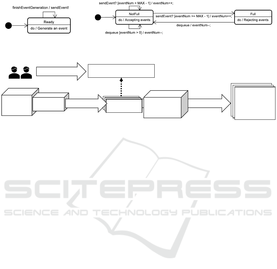
(a) Event generator. (b) Event queue.

Figure 1: State machine model using the concepts of glossary, communication and script.

Model

editor

Extension

[Proposed]

Property Notation

conform to

[expected]

Developers

1. Create

[manually]

[automatically]

3. Output

Diagram

Generator

[Proposed]

Edit log

2. Output

[automatically]

Property

Lifecycle

Diagram

Property

Lifecycle

Diagram

Property

Lifecycle

Diagram

[Proposed]

Figure 2: Overview of the proposed method.

ues for enabling developers to intuitively trace the

changes in the property values of the same state ma-

chine diagram. Furthermore, we have integrated the

proposed method with a method to add a glossary,

etc. to the state machine diagram notation (Ogata

and Kayama, 2019), so that developers can determine

whether property values conform to a glossary, etc.

This study aimed to answer the following research

question: “what clues can the lifecycle of properties

provide to understand the changes of the diagram?”.

To achieve this aim, we have preliminary evaluated

the proposed method by applying it to the edit log by

10 computer science students.

The contributions of this paper are as follows:

• Originality: The property lifecycle diagram was

proposed and then evaluated in the evaluation for

the proof of concept.

• Effectiveness: As an experimental result, the

proposed method enabled experimenters to intu-

itively trace the changing state machine diagrams.

For instance, they identiﬁed the participants who

misunderstood where to give terms, could not ac-

curately use terms or changed their understand-

ings in the middle of modeling, as the result of

interpreting the traces.

2 BASICS OF UML STATE

MACHINE DIAGRAM

Figure 1 presents sample UML state machine dia-

grams in a model. A rectangle with rounded corners

indicates a state. A state can have the following prop-

erties: name, do-activity and entry and exit actions.

In Figure 1, NotFull is the state name, and do /

Accepting events is the do-activity that describes

the behaviors during a stay in a state. An open ar-

rowhead line indicates a transition. A transition can

have the following properties: trigger, guard and ef-

fect. Figure 1, dequeue presents an example of a trig-

ger that corresponds to an event, and [eventNum >

0] presents an example of a guard that describes tran-

sition conditions. Moreover, /eventNum--; presents

an example of an effect describing behaviors during a

traverse of the transition. A ﬁlled circle indicates an

initial pseudo-state as an entry point.

3 PROPOSED METHOD

Figure 2 presents an overview of the proposed

method. The edit event types triggering the logging of

the model ﬁle in editing are create, update, delete

and move as shown in Table 1. Each logged ﬁle is

named by Unix time that indicates the time of log-

ging the ﬁle. For the logged model ﬁles called an edit

log, the proposed method analyses the difference in

each pair of model ﬁles adjacent in the time series.

3.1 Property Lifecycle Diagram

A property lifecycle diagram takes the form of a state

transition diagram and visualizes the lifecycles for

properties. The lifecycle means that the change his-

tory of property values from creating the property un-

til deleting it. A property lifecycle diagram shows the

lifecycle integrating the lifecycles of the same type of

properties extracted from all the diagram elements. In

MDI4SE 2021 - Special Session on Model-Driven Innovations for Software Engineering

522

(delete)

traverse 2

stay=2 end=0

stay=1 end=0

stay=1 end=1

traverse 1

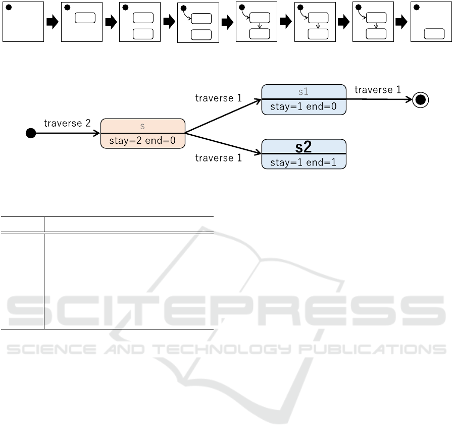
Figure 3: Edit log.

Figure 4: Property lifecycle diagram for state name.

Table 1: Edit Event Types Triggering Logging.

Type Description

create A new vertex or transition was created.

delete Existing vertices and/or transitions

were deleted.

update Properties such as a state name were

updated.

move Existing vertices and/or transitions

were moved.

other words, A property lifecycle diagram is created

for each type of property, i.e., state name, do-activity,

entry and exit actions, trigger, guard, and effect.

Figure 3 shows a simple example of an edit log

starting with the snapshot SS

. In this log, an initial

pseudo-state and two states were initially created. The

initial names of these two states are the same name

s. A transition then was created between the initial

pseudo-state and one state. Furthermore, a transition

was created between those two states. The names of

those two states then were changed to s1 and s2, re-

spectively. Finally, the state s1 has been deleted.

Figure 4 shows the property lifecycle diagram for

the state names in the edit log of Figure 3. In this dia-

gram, a ﬁlled circle indicates that properties were cre-

ated. Meanwhile, a ﬁlled circle surrounded by a circle

indicates that properties were deleted. With regard

to a rectangle with rounded corners, the top region

shows a property value, and the bottom region shows

the passage information. stay means the number of

times that the property value, e.g., s, was assigned to

the property due to some change. For instance, the

name s is assigned to state name properties twice

in total in Figure 4. Thus, the corresponding stay

is 2. end indicates the number of the values that ap-

peared in the last model in the edit log. For instance,

the end for s2 is 1, since it only appeared once in the

last model, i.e., SS

. If the end is one or more, the

font of the property value becomes bold and large. If

not, the font becomes grey.

Meanwhile, an arrow indicates changes in the

property value. For instance, there is the arrow from

s to s1 because the name of one state s was changed

to s1 between SS

and SS

. traverse denotes the

number of times that the property has been changed

from the source value, e.g., s, to the target one, e.g.,

s1. For this arrow, traverse is 1 since the change

only occurred once.

A rectangle with a blue background indicates that

the property value conformed to the corresponding

property notation. Contrarily, red means that the

value did not conform to the property notation. If no

property notation exists, all rectangles always have a

blue background. The method proposed in our pre-

vious study can check whether property values con-

form to the property notation automatically (Ogata

and Kayama, 2019). There are three types of nota-

tion element: glossary; communication; and script.

The glossary is a set of terms. The communica-

tion synchronizes behaviors between different tran-

sitions. The script is executable code handling vari-

ables. However, those details are omitted in this paper

due to limited space.

3.2 Property Lifecycle Diagram

Generation from Edit Log

Property lifecycle diagrams are generated from the

differential analysis results for each pair of model

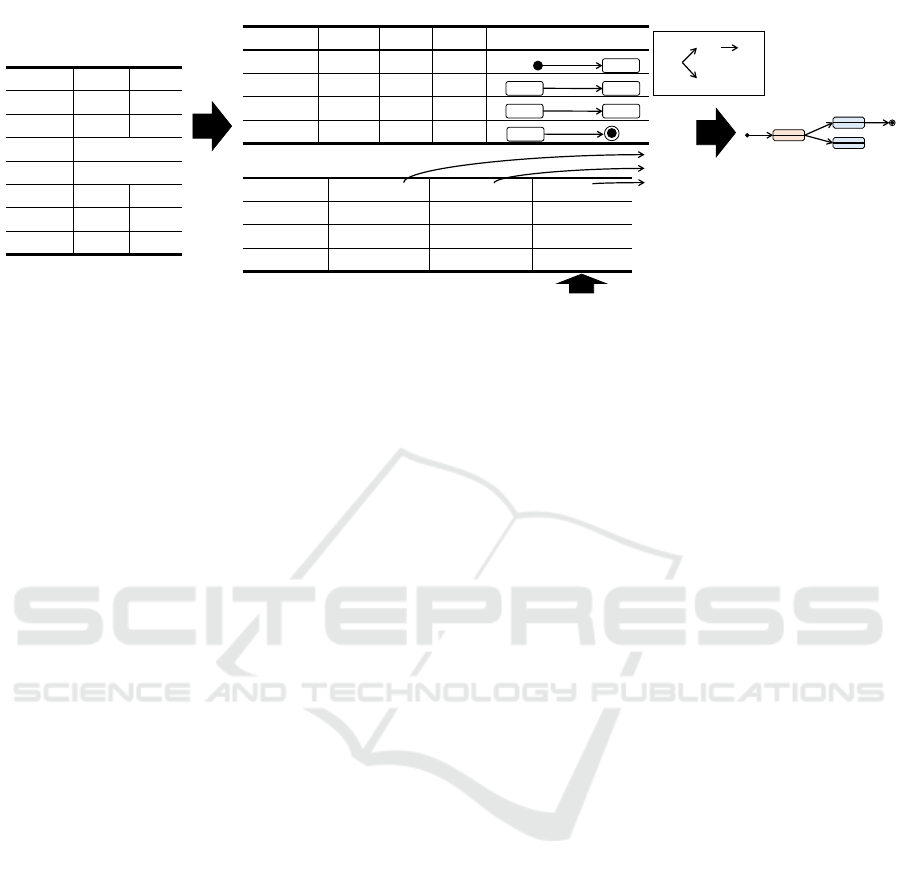
ﬁles adjacent in the time series. Figure 5 shows an

overview of a property lifecycle diagram generation

Property Lifecycle Diagram for Tracing State Machine Diagram Changes

523

Pair Before After

- SS

(none) s

- SS

(none) s

- SS

No difference

- SS

No difference

- SS

s s1

- SS

s s2

- SS

s1 (none)

Differences in State Name

between Adjacent Model Files

Fragment Before After Freq. Part

f1 (none) s 2

f2 s s1 1

f3 s s2 1

f4 s1 (none) 1

stay

traverse 2

traverse 1

s1s

traverse 1

s2s

traverse 1

State Name Freq. "After" Freq. "Last"

Conformance

s 2 0 False

s1 1 0 True

s2 1 1 True

*1 The "Last" means SS

in this example.

Information of State Name

Fragments of Property Lifecycle Diagram for State Name

end

Property Notation {"s1", "s2"}

color

Analyze

Merge

traverse 2

stay=2 end=0

stay=1 end=0

stay=1 end=1

traverse 1

Property Lifecycle Diagram

Figure 5: Property lifecycle diagram generation.

based on the example of Figure 3. The left of Fig-

ure 5 shows a result of the differential analysis for

the state name. “Pair” indicates model ﬁles adjacent

in the time series. “Before” indicates the situation of

the former diagram, e.g., SS

, in the difference while

“After” indicates the situation of the latter one, e.g.,

. “(none)” means that the state name did not exist

in the former diagram but exist in the latter one, and

vice versa. “s”, “s1” and “s2” indicate state names.

“No difference” means that the pair was not related to

the difference in the focused property type, e.g., state

name.

The top middle of Figure 5 shows the fragment

list extracted from the result of the differential analy-

sis. A fragment corresponds to an arrow in property

lifecycle diagrams and is identiﬁed uniquely by the

pair of “Before” and “After”. In the left of Figure 5,

there were two rows in which “Before” and “After”

are “(none)” and “s”, respectively. Thus, a fragment

“f1” shows the result of integrating the data of these

two rows. The “Before” value is transformed into the

source rectangle. In the case of “(none)”, it is trans-

formed into a ﬁlled circle. Meanwhile, the “After”

value is transformed into the target rectangle. In the

case of “(none)”, it is transformed into a ﬁlled cir-

cle surrounded by a circle. “Freq.” indicates the fre-

quency that the same fragment appeared in the dif-

ferential analysis result, and becomes the “traverse”

value. Furthermore, the graph of a property lifecycle

diagram can be generated by merging each fragment

pair in which the “After” value in one fragment is the

same as the “Before” value in the other one.

The bottom middle of Figure 5 shows the infor-

mation of state names related to the result of the dif-

ferential analysis. “State Name” indicates the state

names that appeared in the differential analysis result.

“Freq. “After”” indicates the frequency that each state

name appeared in the “After” column of the differen-

tial analysis result. Its value becomes the “stay” value

in the corresponding rectangle in property lifecycle

diagrams. “Freq. “Last”” indicates the frequency that

each state name appeared in the last model ﬁle. Its

value becomes the “end” value. In this example, The

“Last” model ﬁle means SS

in Figure 4. “Confor-

mance” indicates whether each state name conformed

to the corresponding property notation. Its value be-

comes the background color, i.e., blue or red.

3.3 Prototype Tool

To support the proposed method, we have developed

a prototype tool in Java. This tool uses Astah profes-

sional (Change Vision, 2020) for the logging and dif-

ference analysis and PlantUML (Plant UML, 2021)

and GraphViz (Ellson et al., 2004) for the visualiza-

tion. The Astah professional tool is an extensible

model editor and provides Java API for reading and

writing models. The PlantUML tool is a tool to ren-

der model diagrams based on texts in the PlantUML

notation and partially uses the GraphViz tool to deter-

mine the model layout.

4 PRELIMINARY EVALUATION

In this study, we have evaluated the proposed method

to answer the following research question: “what

clues can the lifecycle of properties provide to under-

stand the changes of the diagram?” In this evaluation,

we discussed how the proposed method can be useful

in practice based on the results of applying the pro-

posed method to learners’ edit logs.

MDI4SE 2021 - Special Session on Model-Driven Innovations for Software Engineering

524

4.1 Overview

In this evaluation, each participant created a state ma-

chine model for each of the four modeling tasks in 1

day. There were a total of 11 participants, and each

of them was either a fourth-year undergraduate or

ﬁrst- or second-year graduate computer science stu-

dent. They used the prototype tool for logging their

edit logs. Each participant saved the four models pre-

sented in Table 2 in one ﬁle and submitted the ﬁle,

and then the edit logs were anonymized according to

the experimenter’s instruction. The requirements and

property notations in the modeling tasks were orig-

inally written in Japanese. However, all the models

in one ﬁle were written in English. Hence, the ex-

perimenters excluded that ﬁle from the 11 ﬁles. It is

because the ﬁle made it impossible to validly verify

many property values in the ﬁle based on the corre-

sponding property notations.

4.2 Tasks

There were four modeling tasks. Here, we present the

ﬁrst two due to space constraints. The theme of the

ﬁrst task (Task 1) was a stopwatch. In this task, the

experimenters introduced only a glossary of terms to

the property notation.

• The stopwatch has the left and right buttons.

• The stopwatch is initially stopped.

• The stopwatch begins measuring the time when

the right button is pressed and pauses the measur-

ing time when the right button is pressed again.

• The stopwatch that paused resumes measuring the

time when the right button is pressed.

• The stopwatch that is measuring the time keeps a

lap when the left button is pressed.

• The stopwatch that is not measuring the time re-

sets the time when and the left button is pressed.

• The stopwatch is stopped after a reset.

The theme of the next task (Task 2) was train

boarding. In this task, the experimenters introduced

a glossary and the script to the property notation.

• The variables cntTrain and passenger must be

utilized in this task.

• The number of passengers, i.e. passenger, on the

train is initially zero.

• The number of train vehicles, i.e. cntTrain, is

initially one.

• The train will have a maximum of four vehicles.

• The maximum number of passengers is ﬁve per

vehicle.

• The train can connect one vehicle by one connec-

tion.

• The train can disconnect one vehicle by one dis-

connection when the rest of the vehicles have the

capacity to accommodate all passengers at the

time of the disconnection.

• The train can depart at any time, regardless of the

number of passengers.

• The train will arrive at the next station after a de-

parture.

• The getting on or off the train or the connection or

disconnection of the train can be done only when

the train stops.

4.3 Steps

The experimenters proceeded with the evaluation as

follows:

1. The experimenters elucidated how to write a state

machine model to all the participants.

2. The experimenters conﬁrmed through the partici-

pants’ answers that all of them had the necessary

knowledge to perform all the tasks.

3. Each participant worked on each task at the corre-

sponding limited time. Furthermore, each partic-

ipant also left notes concerning the difﬁculties in

his/her modeling for each task.

4. The experimenters collected the anonymized arte-

facts of all the participants.

5. The experimenters excluded one artefact, since its

type of natural language did not conform to the

property notations.

6. The experimenters visualized the obtained arte-

facts using the proposed method to infer learners’

errors. They also conﬁrmed the notes describing

the participants’ difﬁculties.

4.4 Results

Figure 6 and 7 present the property lifecycle diagrams

of the triggers and guards in Task 1, respectively. The

edit logs of the 10 participants were integrated by

each of these diagrams. The property notation for

triggers in Task 1 accepted the terms left button,

right button and (empty string). It should be

noted that the empty value was shown as , depend-

ing on a prototype tool constraint. Figure 7 indicates

that there was a participant who misunderstood that

those terms for effects, e.g. reset and keep a lap,

Property Lifecycle Diagram for Tracing State Machine Diagram Changes

525

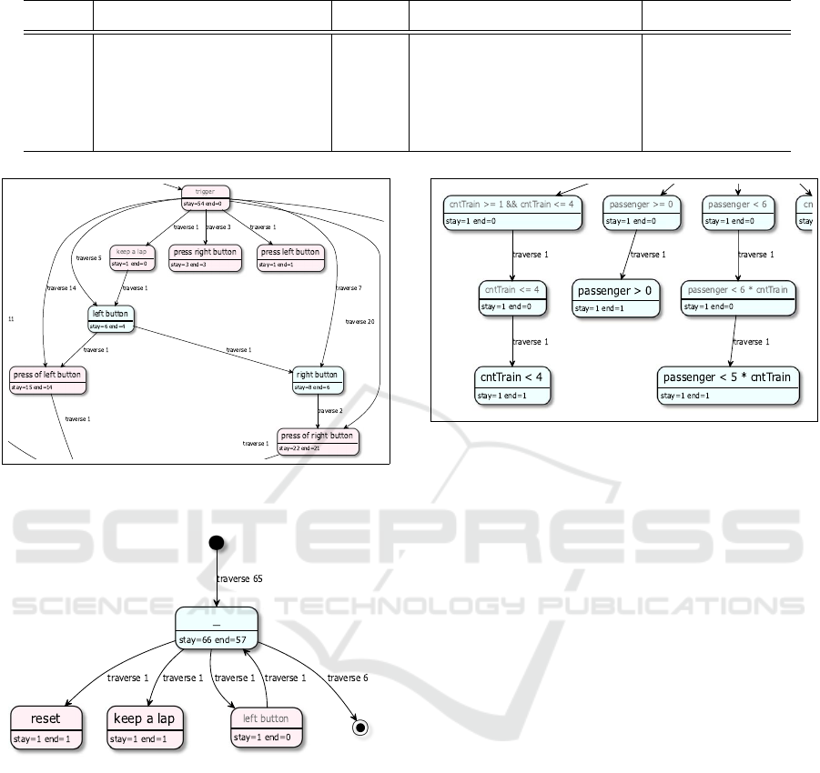
Table 2: Tasks in Evaluation.

ID Concept Time Theme Diagram quantity

Task 1 Glossary 10 min. Stopwatch 1

Task 2 Glossary and Script 20 min. Train Boarding 1

Task 3 Glossary and Communication 20 min. Remote Key Lock 2

Task 4 All concepts 25 min. Producer-Consumer Problem 3

Figure 6: Lifecycle of trigger integrating the edit logs of the

10 participants in Task 1 (excerpt).

Figure 7: Lifecycle of guard integrating the edit logs of the

10 participants in Task 1.

should be utilized for guards. Figure 8 presents the

property lifecycle diagrams of the guards in Task 2.

This diagram indicates the edit log of a participant.

The property notation in Task 2 accepts the script in

the guards and effects at least.

The number of the generated property lifecycle di-

agrams was 539 in total, i.e. 7 properties * (10 par-

ticipants + 1 integration) * 7 state machine diagrams.

Such generation result raised a issue: is it difﬁcult to

grasp the generated diagrams that integrate the edit

logs of the 10 participants from the viewpoint of its

complexity? This issue is important since developers

create and maintain a large and complex model usu-

ally.

Figure 8: Lifecycle of guard based on the edit log of a par-

ticipant in Task 2 (excerpt).

With regard to this issue, we investigated the va-

riety of property values. The more the expressions of

the recorded property values, the more the rectangles

and arrows, and thus, the less readable the property

lifecycle diagrams are. Hence, the reduction of the

variety of property values enables developers and re-

searchers to obtain property lifecycle diagrams that

are easy for them to understand. For this reason,

we further investigated how the presence or absence

of a property notation inﬂuences the diversity of the

property values. In this evaluation, six out of seven

types of state machine diagrams, e.g. stopwatch and

train, provided only a glossary for the do activity

properties. Meanwhile, the six types of state ma-

chine diagrams did not provide any property nota-

tion for the state name properties. In other words,

those diagrams accepted free-writing of the state

name properties. Thus, we compared the property

lifecycle diagrams between the state name and do

activity properties and dealt with the six property

lifecycle diagrams for each of the state name and

do activity properties. Furthermore, each set of

the six diagrams corresponds to the six types of state

machine diagrams previously mentioned. We also

handled the property lifecycle diagrams integrating

the edit logs of the 10 participants and visualized the

statistics of those diagrams using a box plot.

Figure 9 presents the box plot indicating the statis-

tics of rectangles and arrows in the property lifecycle

MDI4SE 2021 - Special Session on Model-Driven Innovations for Software Engineering

526

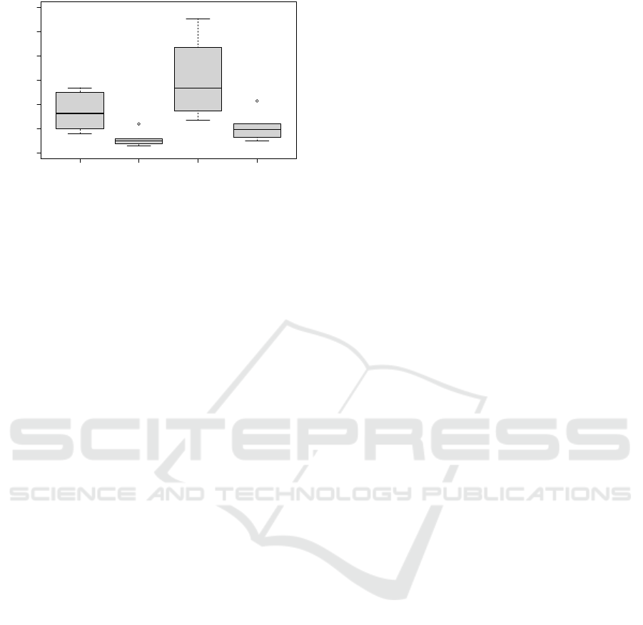
name_rectangle do_rectangle name_arrow do_arrow

0 20 40 60 80 100 120

number of property lifecycle diagram elements

Figure 9: Comparison of the statistics of rectangles and ar-

rows in the property lifecycle diagrams between the state

name and do activity properties (N=6).

diagrams. For the labels of the x-axis, name and do

denote state name and do-activity, respectively.

The label of the y-axis denotes the number of prop-

erty lifecycle diagram elements. As can be seen from

Figure 9, the do activity property, which provides a

glossary, had a signiﬁcantly lower number of rectan-

gles and arrows as well as variations compared with

the state name, which does not provide a property no-

tation. This ﬁnding indicates that the property lifecy-

cle diagrams of the do activity property are small

and simple, to the extent that researchers and educa-

tors can easily grasp the entire diagrams.

4.5 Discussion on RQ: What Clues Can

the Lifecycle of Properties Provide

to Understand the Changes of the

Diagram?

As can be seen from Figure 6, there are some partic-

ipants’ errors in the diagram. A participant deﬁned

a trigger with keep a lap, which is a term for the

effect but not the trigger. The participant likely mis-

understood the correspondence between the property

notation and properties at the beginning. However, in

the ﬁnal models, this error did not exist because the

participant was able to ﬁx it. What is worse is that,

as can be seen from Figure 7, the participants seem to

have left the wrong deﬁnition intact due to their as-

sumptions. They have written property values in the

guard what should be in the effects or triggers. A par-

ticipant has noticed and removed one of the errors.

These ﬁndings suggest that developers will have the

opportunity to learn about past failed designs from the

property lifecycle diagram and thus will be less likely

to make the same mistakes. These ﬁndings also can

only be obtained by analyzing the editing logs.

As can be seen in Figure 8, the participants

changed the guard several times and seemed to have a

hard time deﬁning the guard. For instance, this is sim-

ilar to where developers encounter difﬁculties in tun-

ing parameters. Knowing where was changed many

times by using the property lifecycle diagram leads

developers to understand speciﬁcations that are difﬁ-

cult to determine. It is also difﬁcult for developers to

know without analyzing the process through edit logs,

etc.

Meanwhile, as can be seen from Figure 9, the vari-

ety of the do activity property was explicitly lower

than the state name property. Since each state has

both properties, the numbers of properties analyzed

are the same for both property lifecycle diagrams.

The number of rectangles that the end value was over

0 was 31 for the do activity properties and 77 for

the state name properties. Since the input method is

the use of a keyboard, the risk of careless mistakes is

considered to be similar for both properties. Thus, the

provision of property notation seems to have reduced

the variety of property values. Therefore, the use of

the property notation reduces the number of noisy de-

scriptions and thus avoids unnecessarily complicated

and large-scale change histories, which is considered

to improve the quality of traceability.

Although property lifecycle diagrams can provide

useful information to developers as explained above,

they may become complex and large with the size of

the edit log even if the property notation aids devel-

opers in reducing the variety of words. Therefore, it

is desirable to obtain appropriate feedback through

quantitative analysis, however, the establishment of

this method is future work.

5 CONCLUSION AND FUTURE

WORK

This paper has presented a property lifecycle diagram

and a method to generate it from the edit log of a state

machine model. In a large-scale project, the number

of traceability links becomes enormous and difﬁcult

to manage. A conventional straightforward represen-

tation of the links in the form of a matrix can be a

means of management, however, it may be difﬁcult to

trace the changes in speciﬁc values. As shown in the

preliminary evaluation results, the proposed method

is potentially useful for tracing and understanding the

changes in property values.

As future work, we consider how to use the

property lifecycle diagrams for impact analysis. To

achieve this goal, we will attempt to analyze the

property lifecycle diagram quantitatively and also

combine the proposed method with existing methods

(Kchaou. et al., 2017). The proposed method can be

Property Lifecycle Diagram for Tracing State Machine Diagram Changes

527

combined with various existing methods for traceabil-

ity since the concept of the proposed method can be

applied to different types of diagrams. To deal with

the complexities of the logs, we also plan to use pro-

cess mining tools such as Disco (Fluxicon, 2021) that

can narrow activities and paths in a lifecycle model.

ACKNOWLEDGEMENTS

This work was supported by JSPS KAKENHI Grant

Numbers JP16H03074 and JP20K03146.

REFERENCES

Agner, L. T. W., Soares, I. W., Stadzisz, P. C., and Simao,

J. M. (2013). A brazilian survey on uml and model-

driven practices for embedded software development.

Journal of Systems and Software, 86(4):997–1005.

Change Vision (2020). Astah. http://astah.net/. Last ac-

cessed on Feb. 24, 2021.

Ellson, J., Gansner, E. R., Koutsoﬁos, E., North, S. C., and

Woodhull, G. (2004). Graphviz and dynagraph - static

and dynamic graph drawing tools. In J

unger, M. and

Mutzel, P., editors, Graph Drawing Software, pages

127–148. Springer.

Fluxicon (2021). Disco. https://ﬂuxicon.com/disco/. Last

accessed on Mar. 23, 2021.

Foster, S., Nemouchi, Y., O’Halloran, C., Stephenson, K.,

and Tudor, N. (2020). Formal model-based assurance

cases in isabelle/sacm: An autonomous underwater

vehicle case study. In Proceedings of the 8th Inter-

national Conference on Formal Methods in Software

Engineering, FormaliSE ’20, page 11–21, New York,

NY, USA. Association for Computing Machinery.

Graja, I., Kallel, S., Guermouche, N., Cheikhrouhou, S.,

and Hadj Kacem, A. (2018). A comprehensive sur-

vey on modeling of cyber-physical systems. Con-

currency and Computation: Practice and Experience,

page e4850.

Heisig, P., Stegh

ofer, J.-P., Brink, C., and Sachweh, S.

(2019). A generic traceability metamodel for enabling

uniﬁed end-to-end traceability in software product

lines. In Proceedings of the 34th ACM/SIGAPP

Symposium on Applied Computing, SAC ’19, page

2344–2353, New York, NY, USA. Association for

Computing Machinery.

Horv

ath, B., Graics, B., Hajdu, A., Micskei, Z., Moln

ar,

V., R

ath, I., Andolfato, L., Gomes, I., and Karban, R.

(2020). Model checking as a service: Towards prag-

matic hidden formal methods. In Proceedings of the

23rd ACM/IEEE International Conference on Model

Driven Engineering Languages and Systems: Com-

panion Proceedings, MODELS ’20, New York, NY,

USA. Association for Computing Machinery.

Huang, C.-H., Hsiung, P.-A., and Shen, J.-S. (2010). Uml-

based hardware/software co-design platform for dy-

namically partially reconﬁgurable network security

systems. Journal of Systems Architecture, 56(2):88–

102.

Kan, S. and Huang, Z. (2018). Detecting safety-related

components in statecharts through traceability and

model slicing. Software: Practice and Experience,

48(3):428–448.

Kchaou., D., Bouassida., N., and Ben-Abdallah., H. (2017).

A new approach for traceability between uml models.

In Proceedings of the 12th International Conference

on Software Technologies - Volume 1: ICSOFT,, pages

128–139. INSTICC, SciTePress.

Kraemer, F. A., Slatten, V., and Herrmann, P. (2009). Tool

support for the rapid composition, analysis and imple-

mentation of reactive services. Journal of Systems and

Software, 82(12):2068–2080.

Object Management Group (2017). Uniﬁed modeling lan-

guage 2.5.1. https://www.omg.org/spec/UML/2.5.1/

PDF. Last accessed on Feb. 24, 2021.

Ogata, S. and Kayama, M. (2019). SML4C: fully automatic

classiﬁcation of state machine models for model in-

spection in education. In Burgue

no, L., Pretschner,

A., Voss, S., Chaudron, M., Kienzle, J., V

olter,

M., G

erard, S., Zahedi, M., Bousse, E., Rensink,

A., Polack, F., Engels, G., and Kappel, G., editors,

22nd ACM/IEEE International Conference on Model

Driven Engineering Languages and Systems Compan-

ion, MODELS Companion 2019, Munich, Germany,

September 15-20, 2019, pages 720–729. IEEE.

Pencheva, E. and Atanasov, I. (2016). Engineering of web

services for internet of things applications. Informa-

tion Systems Frontiers, 18(2):277–292.

Plant UML (2021). Plant uml. https://plantuml.com/. Last

accessed on Feb. 24, 2021.

Sanden, B. and Zalewski, J. (2006). Designing state-based

systems with entity-life modeling. Journal of Systems

and Software, 79(1):69–78.

Sulaiman, R., Jawawi, D., and Halim, S. A. (2020). Fea-

tures and behaviours mapping in model-based testing

in software product line. IOP Conference Series: Ma-

terials Science and Engineering, 884:012052.

Vidal, E. J. and Villota, E. R. (2018). Sysml as a tool for

requirements traceability in mechatronic design. In

Proceedings of the 2018 4th International Conference

on Mechatronics and Robotics Engineering, ICMRE

2018, page 146–152, New York, NY, USA. Associa-

tion for Computing Machinery.

MDI4SE 2021 - Special Session on Model-Driven Innovations for Software Engineering

528