
A Comparison of Interpolation Techniques in Producing a DEM
from the 5 m National Geospatial Institute (NGI) Contours
Prevlan Chetty and Solomon Tesfamichael
Department of Geography, Environmental Management and Energy Studies,
University of Johannesburg, Johannesburg, South Africa
Keywords: GIS, Remote Sensing, Interpolation, LiDAR, Kriging, Inverse Distance Weighting, Spline, Nearest
Neighbour, Topo to Raster, ANUDEM, Chief Directorate National Geospatial Information, NGI.
Abstract: Continuous elevation surfaces, which are commonly referred to as Digital Elevation Models (DEM), are vital
sources of information in flood modelling. Due to the multitude of interpolation techniques available to create
DEMs, there is a need to identify the best suited interpolation techniques to represent a localised hydrological
environment. This study investigated the accuracies of commonly applied interpolation techniques including
Inverse Distance Weighting (IDW), Nearest Neighbour (NN), Kriging, Spline and Topo to Raster
interpolation techniques as applied to a 5-m interval elevation contours as a precursor to simulate a flood zone
in the Roodepoort region in Johannesburg, South Africa. A 50 cm resolution DEM derived from aerial Light
Detection and Ranging (LiDAR) point cloud was used as a reference to compare the five interpolations
techniques. The Topo to Raster results were not significantly different from the reference data (P = 0.79 at
95% confidence level), where elevation values were on average underestimated by 0.93 m. In contrast, the
spline interpolation showed the highest significant difference from the reference data (P = 0.00 at 95%
confidence level), with an average underestimation of the elevation by 69.84 m. Outlier identification using
standardized residual analysis flagged significant elevation outliers that were produced in the interpolation
process, and it was noted that most of the outliers across all techniques coincide with areas that showed
frequent topographical changes. Specifically, the largest significant differences using the Topo to Raster
technique were overestimations of the elevation that occur in the upstream section of the tributary. The Spline
technique in contrast showed significant underestimations of the elevation throughout the river system.
Overall, the results indicate that the Topo to Raster technique is preferred to accurately represent the
topography around a river system of the study area.
1 INTRODUCTION
Flooding is a globally occurring phenomenon that
causes property loss and casualties all around the
world (Teng et al., 2017). A flood is characterised by
an overflow of water that submerges land that would
usually be dry which is often referred to as the flood
inundation area (Merz and Blöschl, 2008). The extent
to which a given river will flood to is commonly
referred to as a flood-line (the maximum extent of the
flood inundation area) and is related to the effect that
a specific volume of water has on a hydrological
system through rainfall events (Nkwunonwo et al.,
2020). The statistical likelihood of a rainfall volume
is commonly translated to 10-Year, 50-Year and a
100-Year, and a flood event (Smithers, 2012). As part
of South Africa’s Council for Scientific and Industrial
Research’s (CSIR) Guidelines for Human Settlement,
Planning and Design (CSIR, 1999), no urban
development should be allowed in the demarcated 50-
year flood-line extent. The requirement itself
originates from the National Building Regulation and
Building Standards Act of South Africa (Act 103 of
1997) and is solely based on safety considerations.
The establishment of the flood-line extents therefore
play a crucial role in any development along a river.
In deterministic computer aided techniques of
demarcating a flood-line, one of the most important
aspects is the input elevation data that defines the
geometry of the river and its surrounding basin
(Saksena & Merwade, 2015). Flood-line mapping
often produces results that vary with different sources
of elevation data. The outputs are affected by the
vertical accuracy which is determined by the
Chetty, P. and Tesfamichael, S.
A Comparison of Interpolation Techniques in Producing a DEM from the 5 m National Geospatial Institute (NGI) Contours.
DOI: 10.5220/0010525100370047
In Proceedings of the 7th International Conference on Geographical Information Systems Theory, Applications and Management (GISTAM 2021), pages 37-47
ISBN: 978-989-758-503-6
Copyright
c
2021 by SCITEPRESS – Science and Technology Publications, Lda. All rights reserved
37

topography of the region and the spatial resolution of
the elevation data (Li et al., 2010). In addition, the
importance of interpolation algorithm accuracy is
recognised as an integral component in representing
the topography in numerical form (Chaplot et al.,
2006). If interpolation forms an integral component
of defining topography, and the topography forms an
important part of the flood-line process, it can be
inferred that the interpolation procedure of elevation
data plays an important role in the development of
flood-line extents.
For elevation data to be accurately incorporated
into the flood-line modelling process, there needs to
be spatial continuity in the elevation dataset by
creating a raster surface referred to as a Digital
Elevation Model (DEM). DEMs are derived through
the process of interpolation, which refers to the
prediction of a series of unknown values located
between a limited number of sample points (Manuel,
2004). Interpolation techniques, of which numerous
techniques are available, are commonly used for
geographic data that are represented as points or lines
having elevation information. These techniques are
commonly grouped into local/global,
deterministic/geostatistical and exact/approximate
classes (Erdogan, 2009). Local methods of
interpolation include the Inverse Distance Weighting
(IDW) and the Nearest Neighbour (NN) technique.
Geostatistical methods of interpolation include the
kriging method, which uses the spatial location of
data points rather than relying on the elevation
attribute values alone (Arun, 2013). The spline
(sometimes referred to as rubber sheet) method is
mathematical in nature and takes the form of a cubic
equation whereby each known data point has a cubic
equation where all splines pass through (Robinson &
Metternicht, 2003).
Different interpolation techniques applied to the
same set of elevation data can result in varying DEM
outputs (Arun, 2013). There is therefore a need to
evaluate the suitability and accuracy of these
interpolation techniques for a specific data and
purpose. Erdogan (2009) investigated the relative
accuracy of various interpolation algorithms for an
area with high topographical variance in Turkey. The
research evaluated various deterministic interpolation
algorithms against a baseline survey grade dataset.
The best results were obtained using the thin plate
spline algorithm, a derivative of the spline algorithm
itself. Zimmerman et al. (1999) compared the outputs
of the IDW versus the kriging methodology and
showed that the kriging method was able to adjust
itself to the spatial variability of the data and by doing
so, yielded better estimation of altitude for unknown
sample points. In contrast, Aguilar et al. (2005)
presented research from their study area in Almeria,
Spain, that indicated that the IDW method was
marginally better than the accuracy from the kriging
model output.
In 1984, Mark was the first to propose an
algorithm for automatically delineating a drainage
network from DEM data for specific applications in
hydrological modelling (Mark, 1984). This study
gave rise to the need for hydrological correction
algorithms in the DEM interpolation process which
includes the development of the Australian National
University Digital DEM (ANUDEM), known as the
Topo to Raster feature in ArcGIS, to generate
elevation models that are hydrologically conducive to
network extraction (Callow et al., 2007). The
ANUDEM method creates an interpolated surface
that preserves the critical geometry components
required to define a hydrological system which
includes ridgelines and stream networks (Arun,
2013). Pavlova (2017) presented research conducted
in the Omsk region in Russia which evaluated the
outputs from IDW, Kriging, Topo To Raster, Spline,
Nearest Neighbour (NN) and the Triangulated
Irregular Network (TIN) techniques. The findings
indicated that on relatively flat areas, the best results
were obtained using the Spline and IDW techniques.
In a contrasting environment, Salekin et al. (2018)
conducted research into utilising Global Navigation
Satellite Systems (GNSS) as a data source to generate
a DEM in a landscape with a large degree of
topographical variation in Marlborough, New
Zealand. The GNSS data were used in various
interpolation techniques including NN, Topo to
Raster and IDW techniques. The quantitative research
showed that the Topo to Raster technique showed the
most accurate DEM results, while the IDW showed
the least accurate results.
Chaplot et al. (2006) investigated the suitability of
various interpolation techniques across a
mountainous region in Laos and undulating
landscapes in France. The recommendations
following the results of the study indicated that the
accuracy of the various interpolation techniques
needs to be tested in terms of their applicability to
multiple resolution data (Chaplot et al., 2006). Many
studies have been focused on modelling and
identifying the spatial distribution of errors associated
with DEM’s in order to remove DEM errors (Aguilar
et al., 2010; Hu et al., 2009; Stal et al., 2012).
The above studies show that the accuracy of
interpolated elevation is affected by the topography
of the area of interest and the interpolation techniques
used to create the continuous surface. assessment,
GISTAM 2021 - 7th International Conference on Geographical Information Systems Theory, Applications and Management
38
with different interpolation techniques being more
and less effective in varying landscapes. In South
Africa, the Chief Directorate for National Geospatial
Institute (NGI) produces a 5 m resolution elevation
dataset that can be used by the public for different
purposes. There is a significant gap in assessing the
accuracy of the various interpolation outputs based on
the NGI dataset against survey-grade elevation data
sources. The limitations associated with the
application of the 5 m resolution NGI dataset needs
to be understood in terms of the identification of
spatial distribution errors and the circumstances that
lead to these errors. This study therefore aims to
compare various interpolation techniques to derive a
DEM data for the eventual development of flood-
lines using the 5 m NGI elevation contours in the
Roodepoort region in Johannesburg, South Africa.
The specific objectives of the study are to (1) compare
various interpolation techniques conducted on the
NGI elevation data source which includes the IDW,
NN, Kriging, Spline and Topo to Raster techniques
and (2) identify limitations associated with the
interpolation accuracy of the NGI dataset. The
performances of the interpolators will be evaluated
using a high-resolution Light Detection and Ranging
(LiDAR) derived DEM. It is expected that the
comparisons of the various interpolators will
contribute to hydrological modelling in South Africa
by listing recommendations and limitations of the
application of specific interpolation techniques to the
5 m NGI data source for DEM outputs.
2 METHODS
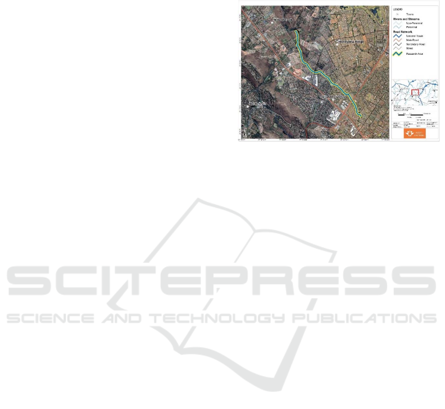
2.1 Study Area
The study area focuses on a 5-kilometre length of a
river that is a tributary of the Wilgespruit River,
between Willowbrook and Strubens Valley in
Roodepoort, Johannesburg (Figure 1). The channel
width ranges from between 5 and 20 m over the length
of the study area and flows seasonally between
October and March (Climate-data.org, 2019). The
study area is composed of an urban residential
composition, which is amongst the highest affected
land-use classes affected by the effects of flooding
(Davis-Reddy et al., 2017).
The Roodepoort region receives approximately
610 mm of rain per year, with the majority occurring
during the summer months from November to
February (Climate-data.org, 2019). The region is
classified as warm and temperate according to the
Köppen and Geiger climate classification (Conradie,
2012). The warmest months by average temperature
are between November and February.
Figure 1: Research Area - Tributary of the Wilgespruit
River, displayed in true colour Red-Greed-Blue (RGB)
band combination.
2.2 Data
2.2.1 5 m Chief Directorate National
Geospatial Contours
The 5 m-resolution contour dataset from the DRDLR
is generated by the Intergraph Dual Mass Camera
(DMC) which captures stereo imagery at a GSD of
0.5 m (NGI, 2018). The NGI also contracts service
providers with similar cameras to acquire data owing
to the scale of the operation. Currently, the NGI aims
to capture 40% of the country every 3 years and the
remaining areas every 5 years. The dataset included
in this research is the 5 m contour dataset (referred to
as the NGI dataset), which was last updated 8
December 2009, for the study area.
The 5 m resolution contour dataset has the largest
spatial coverage compared with more recent high-
resolution survey campaigns that have been
commissioned by the City of Johannesburg (COJ)
Municipality. While higher resolution (that is, to
smaller GSD) datasets are available for metropolitan
areas in South Africa, sites that fall outside of the
metropolitan area demarcations are at best covered by
the 5 m contour offering. As such, the 5 m NGI
dataset is a popular choice among specialists who
seek to apply topographical elements to their
respective studies.
2.2.2 Light Detection and Ranging Point
Cloud
The LiDAR data for the study area was obtained from
the COJ Municipality Corporate Geo-informatics
Department. LiDAR is a popular method of surveying
A Comparison of Interpolation Techniques in Producing a DEM from the 5 m National Geospatial Institute (NGI) Contours
39

that uses an active remote sensing system composed
of at least three sensors, the Inertial Measurement
Unit (IMU), the Global Positioning System (GPS)
and the laser scanner (Csanyi & Toth, 2007). A target
is illuminated by a light source through a laser beam
and the time taken for the reflected beam to return to
the sensor allows for the calculation of survey-grade
measurements relating to the linear position of the
target from the sensor (Vosselman, 2003).
Advancements in optical and computing technologies
have seen the emergence of LiDAR as a rapid and
accurate terrain mapping tool (Lohani & Ghosh,
2017). The COJ municipality region distributes an
aerial-based LiDAR data that is acquired by a
contracted service provider every three years. The
data sourced for this study was acquired in June 2012.
The native format for the LiDAR data includes
American Standard Code for Information Interchange
(ASCII)-based text files that contain information
relating to each point’s location and elevation, which
collectively form a point cloud. The LiDAR point
clouds used in the present study had a point density
of 0.2 points per square meter with an approximate
average spacing between neighbouring points of 2 m.
Therefore, LiDAR is acknowledged for its survey-
grade level of accuracy (Vosselman, 2003; Lohani &
Ghosh, 2017). The horizontal accuracy of the LiDAR
data had a 0.048 m root mean square error (RMSE),
and a vertical accuracy of 0.32 m RMSE as verified
using a network of seven ground control points. The
points were classified into ground and non-ground
points by the data supplier, with the ground points
representing the physical ground level, while the non-
ground points represented all features above ground
including vegetation and structures. The ground
points were used in the present study to serve as the
baseline dataset to evaluate the relative accuracy of
the different interpolation techniques applied to the 5
m elevation contour dataset.
2.3 Analysis
To produce continuous digital representations of a
surface, interpolation techniques were derived to
calculate unknown values that lie between known
values. In this study, five interpolation techniques
conducted on the 5 m resolution NGI dataset were
compared, namely IDW, NN, kriging, spline, and
Topo to Raster algorithms.
IDW is a non-linear, deterministic interpolation
technique that computes a weighted average of a
value from sample points in close vicinity to
determine the value of non-sampled points (Robinson
& Metternicht, 2003). The IDW principle was first
presented by Shepard (1968) for improved efficiency
of the central processing unit time. Today, the IDW
process is one of the most widely applied methods of
interpolation in the hydrological environment. The
IDW principle assumes that values which are close
together are more alike than values that are further
away. To calculate the value of an unknown point at
a location, the weighted average of the surrounding
known values is calculated and assigned to the
unknown point. Known values that are closer to the
location of the unknown point are given a higher
weighting ranking in the calculation, and therefore
have a larger influence on the determination of the
unknown value, opposed to known values that are
further away. Definitions of the neighbouring radius
for the calculation and the power function
representing the inverse distance relationship
between the points are critical parametres for this
interpolation method. The formula for the IDW
interpolation is defined as 𝑍
∑
.
∑
, where 𝑍
= value of variable Z in point I; 𝑍
= the sample in
point I; 𝑑
= distance to the sampled point from the
unknown point; N = coefficient that defines the
weight that will be based on the inverted distance
function; n = total number of predictions allowed for
each validation (Shepard, 1968).
The NN Interpolation model is based on the
Sibson interpolation model, where values are
assigned to un-sampled points based on the
construction of Thiessen polygons which work
together to form areas of overlap (Sibson, 1980). The
polygons are formed across all known values
surrounding the unknown value by connecting all
common values into a network of Thiessen polygons
which represent all known values. A new Thiessen
polygon is then generated over the unknown value,
and the proportion of the overlap between this new
polygon versus the network of intersecting polygons
previously generated define the weighting system to
be used. The formula used for the NN interpolation is
identical to IDW, with the only difference coming
from the method used to calculate the weightings. The
NN interpolation formula is defined as 𝑍
𝑢
∑
λu z
, where λ
u
and u = (x,y) location of
query point (Rukundo & Cao, 2012).
Kriging is a stochastic local interpolation
technique that computes the value of non-sampled
points in a similar way to IDW, with the exception
that there is more control on the weighting system that
determines unknown values based on distance
(Robinson & Metternicht, 2003). The kriging model
GISTAM 2021 - 7th International Conference on Geographical Information Systems Theory, Applications and Management
40

was developed by Danie Krige, who formed the basis
of what would later be called the kriging process in
1951 through research presented in the Journal of the
Chemical, Metallurgical and Mining Society of South
Africa in the 1960s (Cellmer, 2014). Krige (1951)
applied the kriging technique to survey two gold
mines to understand resource estimation based on
borehole data. An ordinary kriging equation is
defined as 𝑍𝑠
∑
λ zs
, where, λ = weights
assigned to each known value, where all weights sum
to a unity which enables unbiased estimations which
are defined as
∑
λ
1. The matrix equation
calculating the weights is defined as C = 𝐴
𝑏
,where 𝐴 = matrix of semi-variance between the
known values; 𝑏 = estimated semi-variances between
the known values and unknown value, represented by
a vector (Krige, 1951; Krige, 1952).
The spline interpolation is a piecewise polynomial
interpolation method that creates a smooth raster
surface from the known sample points using a 2-D
minimum curve technique (Robinson & Metternicht,
2003). The resulting surface passes through all known
sample points. The spline method is mathematical in
nature and takes the form of a cubic equation whereby
each known data point has a cubic equation through
which all splines pass (Robinson & Metternicht,
2003). Jenkins (1927) and Schoenberg (1946) can be
credited with the origins of the spline method of
interpolation. The spline cubic equation is defined as
𝑆
𝑥,𝑦
𝑇
𝑥,𝑦
∑
𝜆
𝑅𝑟
, where 𝑗 =
1,2,… 𝑁, 𝑁 is the number of points, 𝜆
are the
coefficients found by the linear equation solution and
𝑟
is the distance from the point (x,y) to the 𝑗
point
(Meijering, 2002).
ANUDEM is based on a program developed to
ANUDEM is based on a program developed to
interpolate elevation values across a topographical
surface by Hutchinson (1988). The algorithm
generates elevation models that are hydrologically
conducive to network extraction (Callow et al.,
2007). In the 1980s, a study done by Mark (1984)
proposed an algorithm for automatically delineating a
drainage network from DEM data. This study gave
rise to the need for hydrological correction algorithms
in the DEM interpolation process which includes the
development of the ANUDEM. This interpolation
technique provides a compromise between local
interpolation methods such as IDW and global
interpolation methods such as kriging, by allowing
the resultant DEM values to follow abrupt changes in
terrain which include streams, ridges and cliffs, thus
preserving topographical continuity (Pavlova, 2017).
The Topo to Raster interpolation is the only algorithm
featured in ArcGIS that is preferentially applied to
contour datasets. The Topo to Raster interpolation is
defined by the equation 𝐽
𝑓
𝑓
𝑓
𝑑𝑥𝑑𝑦,
where 𝐽
is known as a local interpolation technique
that is well-suited for features with a better resolution.
Then 𝐽
𝑓
𝑓
𝑓
𝑓
𝑑𝑥𝑑𝑦, where 𝐽
is
known to create unrealistically flat surfaces as
commonly seen by global interpolation techniques.
Hutchinson's ANUDEM program revolves around a
compromise between 𝐽
𝑎𝑛𝑑𝐽
as follows: 𝐽
𝑓
0.5 ℎ
𝐽
𝑓
𝐽
𝑓, where ℎ is the spatial
resolution of the output surface model (Hutchinson,
1988).
2.4 Accuracy Assessment
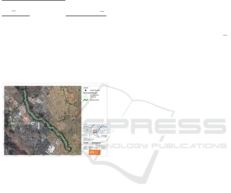
A buffer measuring 100 m was created around the
river’s centreline. Points were then generated at 100
m intervals along the extent of the buffer, from which
LiDAR elevations were extracted within a 5 m
average distance from each point, resulting in a total
of 103 LiDAR spot elevations. Figure 2 shows the
positions of the spot elevation points, plotted against
a 2018 WorldView-2 derived satellite image that is
rendered in red, green and blue (RGB). These
elevation values, along with their X and Y positions,
represent the most accurate remotely sensed dataset
available for this study and were therefore used as
reference data to compare the different surfaces
created using the five interpolators applied to the 5 m
contour data. While a field-collected differential real-
time kinematic GPS system will provide the highest
level of accuracy, the intention of the research
presented is to utilise practical and readily available
datasets, such as the COJ distributed LiDAR.
Elevation values of the five interpolated surfaces
were extracted at each of the above-mentioned
LiDAR spot elevation locations. The T-test and
residual analysis was used to compare the
interpolated surfaces against the baseline LiDAR
elevation values.
2.4.1 Comparing the Output Elevations of
the Interpolated DEMs against the
Reference LiDAR Elevations
The T-test is a statistical procedure that is commonly
used when investigating the relationship between
variables by comparing the means on the dependent
variables against the baseline or independent variable
(Green & Salkind, 2012). The T-test was chosen due
to the flood extent comparisons involved at each
measurement station, where more than one dependent
set of results is be compared to the baseline LiDAR
flood-line extents. The P-value from the T-test output
A Comparison of Interpolation Techniques in Producing a DEM from the 5 m National Geospatial Institute (NGI) Contours
41
is used to assess the degree of difference between the
means of the interpolation elevation versus the
baseline LiDAR elevation. The applied T-test
formula is a generalisation of a two-sample T-test
(Ostertagova & Ostertag, 2013) and is defined as 𝐹
where 𝑀𝑆𝐺
∑
/
and 𝑅𝑀𝑆
∑∑
∑
,
where 𝑌
is the observation distances from the stream
centreline for each output, 𝑇
is the sum of each group
of distances from the stream centreline, G is the total
of all observations being compared for the variance
(model output being assessed versus baseline LiDAR
output), 𝑛
is the number of observations in group i
and n is the total number of observations being
analysed for the variance. The T-test and associated
P-values were calculated using Microsoft Excel
(Microsoft Corporation, 2019).
Figure 2: Location of observations for analysis, displayed
in true colour RGB band combination.
2.4.2 Identification of Outliers from the
Interpolated DEMs against the LiDAR
Reference Data
Analysis of residuals forms part of a regression
analysis which is designed to assess model adequacy
(Martin et al., 2017). Regressions are typically
applied to assess the accuracy of a predicted model
against actual values (Martin et al., 2017). Because
the research purpose is accuracy assessment, as
opposed to model fitting, regression analysis was not
chosen as an accuracy assessment tool in this
research. However, components of the regression
analysis remain useful tools in location-based
analytics, such as the residual analysis which allows
for reference to a specific observation and its
associated spatial location. Residuals are defined as
the vertical distance 𝑟
) between the observed
measurement and the predicted measurement (𝑟
=
𝑦
𝑦., represented by a linear regression line. In
this research, the observed distance (𝑦
) represents the
linear regression from the baseline LiDAR elevation
while the predicted measurement (𝑦) represents the
vertical elevation difference between the
interpolation surface being assessed (Topo to Raster,
kriging, NN, IDW, spline).
Outlier identifications in data have been applied
successfully through the usage of standardised
residuals (Sousa et al., 2012; Miller, 1993, Salekin et
al., 2018) and are defined by the formula 𝑟
,
where the standardised residual (𝑟
) is the residual
value (𝑟
) divided by its standard deviation (𝑠. At a
95% confidence level, it is expected that 95% of the
data falls within 2 standard deviations of the mean
(Sousa et al., 2012). Data points falling lower than -2
and higher than 2 on the standardised residual plot
will therefore represent outliers. The incorporation of
a standardised residual analysis allows for the
identification of interpolated elevation output
observations that are significantly different to the
baseline LiDAR elevation values, which in turn
allows for a spatial expression of the results observed.
The methodology starts with the running of the
various interpolation procedures. As the focus of the
assessment is on the influence of interpolation
techniques on hydrological modelling environments,
a streamflow analysis was run on the baseline LiDAR
dataset, from which a 100 m buffer was generated.
LiDAR points were then selected using proximity
analyses at every 100 m interval along the extent of
the buffer. Interpolated elevation values were then
extracted from each interpolation process at each
LiDAR elevation point every 100 m along the buffer
zone. All GIS-based processing procedures were
conducted using ArcGIS (ESRI, 2019). The
interpolated elevation observations were then
compared against the LiDAR elevations using a T-
test and residual analysis in Microsoft Excel
(Microsoft Corporation, 2019).
A buffer measuring 100 m was created around the
river’s centreline. Points were then generated at 100
m intervals along the extent of the buffer, from which
LiDAR elevations were extracted within a 5 m
average distance from each point, resulting in a total
of 103 LiDAR spot elevations. These elevation
values, along with their X and Y positions, represent
the most accurate remotely sensed dataset available
for this study and were therefore used as reference
data to compare the different surfaces created using
the five interpolators applied to the 5 m contour data.
While a field-collected differential real-time
kinematic GPS system will provide the highest level
GISTAM 2021 - 7th International Conference on Geographical Information Systems Theory, Applications and Management
42
of accuracy, the intention of the research presented is
to utilise practical and readily available datasets, such
as the COJ distributed LiDAR. Elevation values of
the five interpolated surfaces were extracted at each
of the above-mentioned LiDAR spot elevation
locations. The T-test and residual analysis was used
to compare the interpolated surfaces against the
baseline LiDAR elevation values.
3 RESULTS
3.1 Differences between Interpolated
Elevations and LiDAR Elevations
The T-test presented in this section yields information
on the degree of variance between the elevation
values obtained from each interpolation against the
baseline LiDAR elevation values. The T-test was run
at an alpha = 5%. The outputs from the T-test for the
various interpolation algorithms are presented in
Table 1 which has been sorted from most accurate to
least accurate.
The Topo To Raster interpolation had the highest
correlation with the baseline LiDAR elevation with a
P value of 0.75. The lowest P value obtained indicates
a relatively strong correlation to the LiDAR baseline
elevations when compared against the other
interpolation techniques. The mean value from the
Topo to Raster techniques elevation values are close
to the mean value of the LiDAR elevations (1553.99),
with the Topo To Raster interpolation generally
underestimating the elevation by 1.10 m.
The T-test results indicate NN to have the second
highest correlation to the baseline LiDAR elevation
with P value of 0.78. The P value indicates a relatively
good correlation to the LiDAR baseline elevations
when compared against the other interpolation
techniques. The mean value from the NN techniques
elevation values are close to the mean value of the
LiDAR elevations (1553.99), with the NN
interpolation generally underestimating the elevation
by 0.96 m. The Kriging T-test results show this
technique to marginally be the third most accurate
interpolator with results similar to the NN technique
with a P value of 0.79. The IDW T-test results are
within close range of the Kriging and NN
interpolators, showing a relatively good correlation to
the baseline LiDAR elevations with P value of 0.79.
Both Kriging and IDW mean outputs indicate a
general underestimation of the elevation by 0.95 m
and 0.93 m respectively in relation to the LiDAR
mean value.
The spline T-test results show the highest variance
to the baseline LiDAR by far with a P value of 0.00.
The negligible P value and highest mean deviation
from the LiDAR elevation with a general
overestimation of -69.84 m indicate that the spline
interpolation technique is unsuitable for deriving a
suitable DEM from the NGI 5 m dataset.
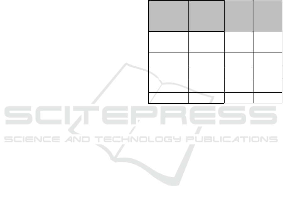
Table 1: T-test results across all interpolation techniques
results. Each interpolation was compared against the
LiDAR mean elevation of 1553.9 m.
Interpolation
Technique
Mean Elevation
(Meters above
mean sea level)
Mean
Difference
between
LiDAR and
Interpolator
(
meter
)
*P Value
Topo To Raster
(
ANUDEM
)
1553.06
0.93
0.754
NN 1553.04
0.95
0.787
Kri
g
in
g
1553.04
0.95
0.787
ID
W
1552.89
1.10
0.791
S
p
line 1623.83
-69.84
0.000
*P value was measured using 95% confidence level
3.2 Identification of Outliers from the
Interpolated DEMs Relative to the
LiDAR Data
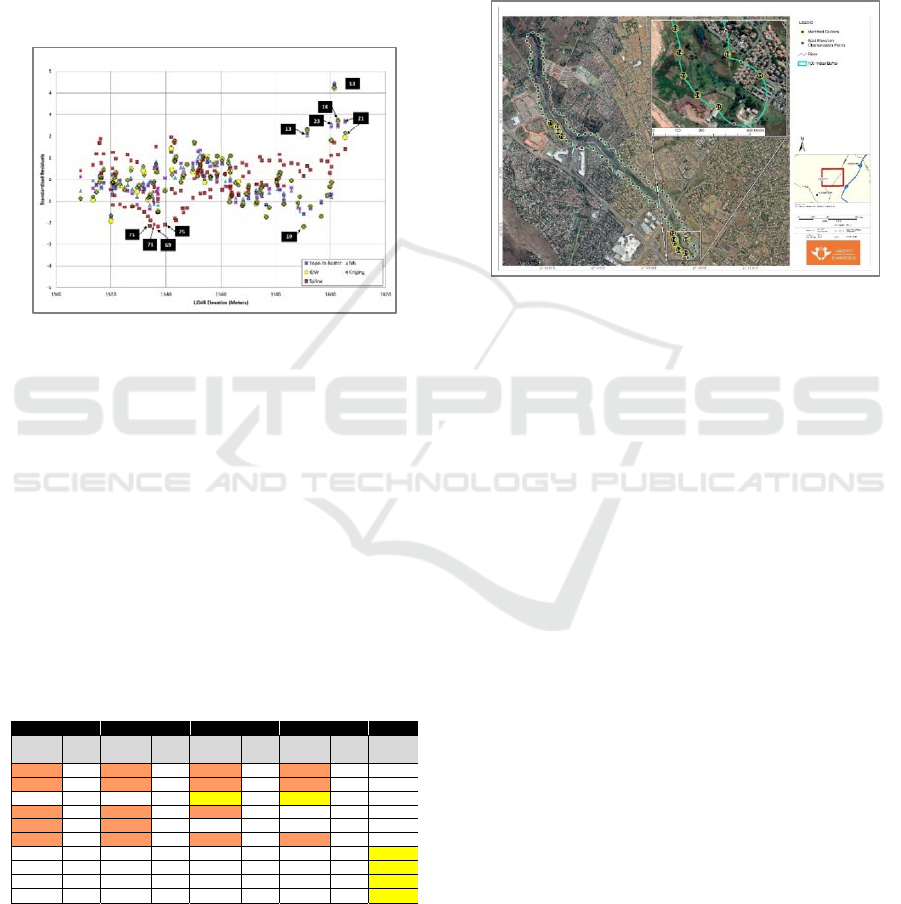
The plotted residual results are presented for each
interpolation technique in Figure 3. The results
graphically illustrate the outliers of significance that
can be related to a spatial location, which forms a
platform for the subsequent discussion around the
results seen. Residuals of Topo to Raster, NN, IDW
and kriging share a similar distribution throughout the
plot. The spline residual plot results resemble the
same general distribution as the other interpolators
but appear to have larger variances along the residual
plot.
The Topo to Raster, NN, kriging and IDW
residual points all show a dependent positive
correlation to the LiDAR elevations with a wave-
form trend about the Y-axis. Elevations of 1500–1540
m and 1560–1600 m show a general underestimation
of elevation values by the Topo to Raster
interpolation. For elevation values of 1540–1560 m,
the Topo to Raster interpolation overestimates the
elevations. Highly significant outliers occur at higher
elevation values at around 1600 m. The IDW and
kriging interpolation outputs have similar
A Comparison of Interpolation Techniques in Producing a DEM from the 5 m National Geospatial Institute (NGI) Contours
43
standardised residual plots, while the Topo to Raster
and NN interpolation outputs share similarities in
their standardised residual plots. The spline
interpolation residual points also show a general
dependent positive correlation to the LiDAR
elevations, but in comparison to the other
interpolators, the spline results have a larger residual
variance. Larger underestimations in elevation values
are seen at 1530–1550 m, with the same general
observation of higher overestimations of elevations at
1600 m.
Figure 3: Combined standardised residuals across all
interpolation techniques with significant outliers identified
with labels.
Table 2 shows the name and location of the
elevation values that were identified through the
residual plot shown in Figure 3. Observations 13, 14,
21, 23 and 24 show overestimations of the elevation
across all interpolation techniques except for the
spline technique. Observation 19 shows
underestimations of elevation in the kriging and IDW
technique while observations 69, 70, 71 and 75 show
underestimations of the elevation only in the spline
technique.
Table 2: Significant outliers Identified from standardised
residual plot analysis.
Figure 4 shows the identified locations of the
significant residual outliers in the upper section of the
tributary (Locations 11, 13, 14, 19, 21, 23 and 24).
The downstream section of the tributary shows a
higher correlation between the LiDAR elevation and
interpolated algorithms that are within a 95%
confidence level of vertical elevation difference. A
large concentration of outliers can be seen in the
upstream section of the tributary, where 5 of the 6
observation outliers identified are overestimations of
elevation. The remainder of residual outliers
identified (69, 70, 71 and 75) are all identified from
the spline interpolation with significant elevation
deviations (all 13 m under the LiDAR elevation).
Figure 4: Identified standardised residual outlier locations,
displayed in true colour RGB band combination.
4 DISCUSSION
The results obtained in the interpolation output
compared against the reference LiDAR data indicate
that the Topo to Raster interpolation technique yields
marginally more accurate DEM surfaces than the
other interpolators, based on the T-test. The Topo to
Raster results agree with existing bodies of research
(Arun, 2013; Salekin et al., 2018) indicating that the
Topo to Raster technique preserves critical
components of the hydrological environment and by
doing so, is the most accurate under these conditions.
The spline interpolation technique was the most
inaccurate and is unsuitable for the application on the
5 m NGI dataset to create a DEM. These results from
the spline methodology are inconsistent with findings
from Erdogan (2009) and Pavlova (2017) who found
that the spline methodology yielded marginally more
accurate results in comparison to other interpolations
assessed. It must, however, be noted that Erdogan
(2009) utilised a thin-plate spline algorithm which is
a derivative of the original spline technique; this was
not used in the research presented here, and Pavlova’s
(2017) findings are representative of an area with low
topographical variations. All other interpolation
techniques assessed in the results presented as part of
this research show good applicability with marginal
differences in variation to the baseline LiDAR.
TopoToRaster NN Kriging IDW Spli
n
Standardised
Residual
Distance
toLiDAR
Elevation
Standardised
Residual
Distance
toLiDAR
Elevation
Standardised
Residual
Distance
toLiDAR
Elevation
Standardised
Residual
Distance
toLiDAR
Elevation
Standardised
Residual
2.14 5.20 2.02 4.91 2.30 5.74 2.29 5.75 0.62
4.39 10.63 4.46 10.83 4.24 10.60 4.22 10.60 1.71
‐1.61 ‐3.90 ‐1.61 ‐3.90 ‐2.16 ‐5.41 ‐2.17 ‐5.44 0.17
2.73 6.62 2.67 6.49 2.15 5.37 1.95 4.89 1.42
2.45 5.93 2.62 6.35 1.82 4.56 1.81 4.55 1.10
2.52 6.12 2.44 5.91 2.74 6.86 2.73 6.85 1.14
‐0.69 ‐1.67 ‐1.18 ‐2.86 ‐1.51 ‐3.77 ‐1.49 ‐3.74 ‐2.17
‐1.06 ‐2.57 ‐1.13 ‐2.74 ‐0.13 ‐0.32 ‐0.12 ‐0.29 ‐2.07
‐1.38 ‐3.34 ‐1.17 ‐2.84 ‐0.80 ‐2.00 ‐0.78 ‐1.97 ‐2.14
0.07 0.17 ‐0.51 ‐1.24 ‐0.54 ‐1.34 ‐0.52 ‐1.31 ‐2.09
GISTAM 2021 - 7th International Conference on Geographical Information Systems Theory, Applications and Management
44
Spatial representations of the outliers as identified
from the residual analysis reveal a large concentration
of points to the upper part of the tributary which fall
on a garden refuse site (Figure 4). Due to the
differences in the temporal acquisition of the data, the
garden refuse site would have undergone
topographical changes to its the baseline LiDAR
(acquired in June 2012) compared to NGI (acquired
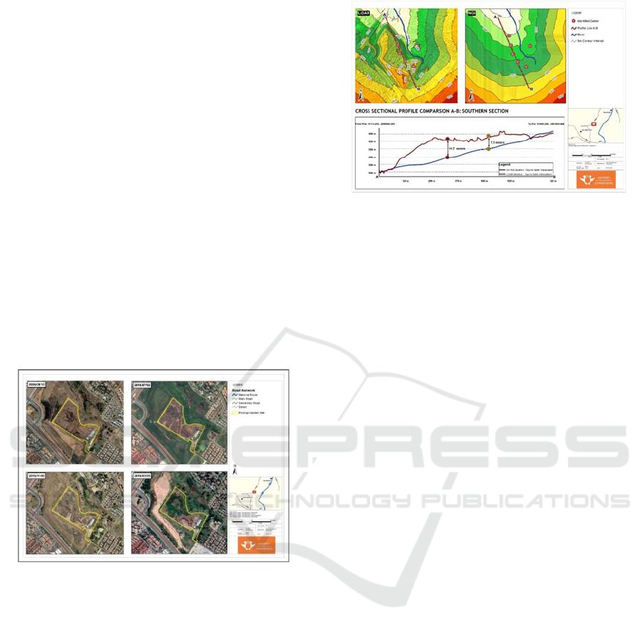
in December 2009). Figure 5 illustrates the
progression of the area, identified as the Weltevreden
Park PickitUp garden refusal site, between 2006 and
2019 which shows the visible changes in topography
over 13 years. Changes in the surface topography
across this site over time have a direct influence on
the elevation values observed during the LiDAR and
NGI data acquisitions. These elevation value
differences are prominent in the residual analysis,
which shows a large concentration of residuals with a
variance larger than 5 m in and around the refuse site.
The residual interpretation further indicates the spline
interpolation’s output is unsuitable for accurate DEM
interpolation from the 5 m NGI data source.
Figure 5: PickitUp garden refuse site surface changes:
2006-2019, displayed in true colour RGB band
combination.
The differences in elevation values between the
NGI versus the LiDAR data reveals large differences
in elevation values in the refuse site region, located in
the upper section of the tributary (Figure 2.7). The
NGI surface along this section is almost constantly
below the LiDAR surface which shows clear
definitions of a dump feature (Figure 2.8). This is
indicative of changes in the surface between the
acquisition of the 5 m NGI dataset (December 2009)
and the LiDAR dataset (June 2012) which is
statistically shown with the underestimation of the
elevation values with the 5 m NGI dataset. The profile
comparisons show a high degree of variance with
regards to topographic changes that have occurred
over the dumpsite, highlighting differences in
temporal resolution as shown in Figure 6.
Figure 6: Profile comparisons for LiDAR (Left) versus NGI
(Right) along A-B.
5 CONCLUSION
The findings of this study indicate that the Topo to
Raster interpolation technique is the most favourable
for the 5 m contour data of the localised study area.
The results also indicate that while the application of
the Topo to Raster technique yielded the most
accurate results, the NN, kriging and IDW techniques
were close to the Topo to Raster technique. These
results imply that the application of the NN, kriging
and IDW interpolation techniques to the 5 m NGI
dataset will yield DEMs with similar vertical
accuracy.
While the results indicate that the Topo to Raster
technique is the most accurate, it must be
acknowledged that certain interpolation techniques
are likely to yield the most favourable results in the
environments for which they were originally
developed. The Topo to Raster interpolation
algorithm was specifically formulated for its
application in hydrological environments
(Hutchinson, 1988), while the geostatistical method
evaluated in this research (kriging) and local methods
(NN and IDW) are limited by the resolution and
spread of data (Al Mashagbah et al., 2012). Research
into the interpolation technique to be applied and its
favourability to different spatial distributions of data
should always be taken into account when
interpolating elevation datasets (Cellmer, 2014). Due
to advancements in technology and information, it is
also likely that the defining geometry (point, line or
polygon) of the elevation data sources may change
from line-based contour elevations to point-cloud
elevation formats, which will also play a significant
role in determining the ideal interpolation technique
to apply.
The results presented in this research are specific
to the application on the freely and nationally
A Comparison of Interpolation Techniques in Producing a DEM from the 5 m National Geospatial Institute (NGI) Contours
45

distributed South African NGI contour dataset. The
residual analysis indicated substantial differences in
elevation between areas for the reference LiDAR and
NGI datasets, which is attributed to differences in
temporal resolution. As access to spatial information
in South Africa increases in association with
advancements in survey techniques, future
assessments should be performed on the most
temporally relevant data available. The findings
indicate that while the usage of lower spatial
resolution datasets such as the 5 m data used in the
present study may be acceptable in terms of RMSE,
the need for access to more temporally relevant
datasets is crucial to accurately represent
topographical information for an area.
REFERENCES
Aguilar, F.J., F. Agu¨era, M.A. Aguilar. & F. Carvajal.
(2005). Effects of terrain morphology, sampling
density, and interpolation methods on grid DEM
accuracy. Photogrammetric Engineering and Remote
Sensing, 71: 805–816.
al Mashagbah, A., R. Al-Adamat. & E. Salameh. (2012).
The use of Kriging Techniques within GIS
Environment to Investigate Groundwater Quality in the
Amman-Zarqa Basin/Jordan. Research Journal of
Environmental and Earth Sciences, 4: 177-185.
Arun, P. V. (2013). A comparative analysis of different
DEM interpolation methods. The Egyptian Journal of
Remote Sensing and Space Sciences, 16(2): 133-139.
Academy of Science of South Africa (ASSAf), (2020).
Quest: Science for South Africa, 16(2).
Callow, J, N., G.S Boggs. & K. P van Niel. (2007). How
does modifying a DEM to reflect known hydrology
affect subsequent terrain analysis? Journal of
hydrology, 332(1-2): 30-39.
Cellmer, R. (2014). The possibilities and limitations of
geostatistical methods in real estate market analyses.
Real Estate and Valuation, 22(3): 54-62.
Chaplot, V., F. Darboux, H. Bourennane, S. Leguedois, N.
Silvera. & K. Phachomphon. (2006). Accuracy of
Interpolation Techniques for the Derivation of Digital
Elevation Models in Relation to Landform Types and
Data Density. Geomorphology, 77: 126-141.
Climate-data.org. (2019). Roodepoort Climate. Available
from https://en.climate-data.org/africa/south-
africa/gauteng/roodepoort-232/.
Conradie, D. C. U. (2012). South Africa’s Climatic Zones:
Today, Tomorrow. International Green Building
Conference and Exhibition, Future Trends and Issues
Impacting on the Built Environment, Sandton, July 25-
26.
Council for Scientific and Industrial Research (CSIR).
(1999). Ecologically Sound Urban Development.
Available from
https://www.csir.co.za/sites/default/files/Documents/
Chapter_05_08_02_-Vol _I.pdf.
Csanyi, N. & C.K. Toth. (2007). Point positioning accuracy
of airborne lidar systems: A rigorous analysis.
International Archives of Photogrammetry, Remote
Sensing and Spatial Information Systems, 36(1):107-
111.
Davis-Reddy, C.L. & K.Vincent. (2017). Climate risk and
vulnerability: A handbook for Southern Africa (2nd
Edition), CSIR, Pretoria, South Africa.
Department of Water and Sanitation (DWS). 2017. The
quaternary drainage regions. Available from
http://www.dwa.gov.za/iwqs/wms/data/000key2data.a
sp.
Erdogan, S. (2009). A comparison of interpolation methods
for producing digital elevation models at the field scale.
Earth Surface Processes and Landforms, 34: 366-376.
ESRI 2019. ArcGIS Desktop: Release 10.7. Redlands, CA:
Environmental Systems Research Institute.
Green, S.B. & N.J. Salkind. (2010). Using SPSS for
Windows and Macintosh: Analysing and understanding
data (5th Edition). Upper Saddle River, New Jersey:
Pearson Education Incorporated.
Hutchinson, M.F. (1988). Calculation of hydrologically
sound digital elevation models, Third International
Symposium on Spatial Data Handling at Sydney,
Australia, vol. 3, no. 1, pp.120–127.
Jenkins, W.A. (1927). Graduation based on a modification
of osculatory interpolation. Trans. Actuar. Soc. Amer,
28:198-215.
Johnson, M. R., C.R. Anhaeusser. & R.J. Thomas. (2006).
The Geology of South Africa. Council for Geoscience.
Krige, D.G. (1951). A statistical approach to some basic
mine valuation problem on the Witwatersrand. Journal
of the Chemical, Metallurgical and Mining Society of
South Africa. 12: 119–139.
Krige, D.G. (1952). A statistical analysis of some of the
borehole values in the Orange Free State goldfield.
Journal of the Chemical, Metallurgical and Mining
Society of South Africa, 9: 47–64.
Lohani, B. & S. Ghosh. (2017). Airborne LiDAR
technology: A review of data collection and processing
systems. Proceedings of the National Academy of
Sciences, India Section A: Physical Sciences,
87(1):567-579.
Manuel, P. (2004). Influence of DEM interpolation
methods in drainage analysis. GIS in Water Resources,
8: 32-28.
Mark, D.M. (1984). Automatic detection of drainage
networks from digital elevation models. Cartographica,
21(2-3): 168-178.
Martin, J., A. David. & A. Garcia Asuero. (2017). Fitting
Models to Data: Residual Analysis, a Primer. Intech.
Available from: http://dx.doi.org/10.5772/68049.
Matheron, G. (1963). Principles of geostatistics. Economic
Geology, 58: 1246-1266.
Meijering, E. (2002). A chronology of interpolation: From
ancient astronomy to modern signal and image
processing. Proceedings of the IEEE, 90(3): 319-342.
GISTAM 2021 - 7th International Conference on Geographical Information Systems Theory, Applications and Management
46

Merz, R. & G. Blöschl. (2008). Flood frequency hydrology:
Temporal, spatial, and causal expansion of information.
Water Resources Research, 3:13-20.
Microsoft Corporation, 2019. Microsoft Excel (Windows
10 version), Available at: https://office.microsoft. com/
excel.
Miller, J.N. (1993). Outliers in experimental data and their
treatment. Analyst, 118(5):455-461.
Nkwunonwo, U.C., M. Whitworth. & B. Baily. (2020). A
review of the current flood modelling for urban flood
risk management in the developing countries. Scientific
African. 7: e00269.
Ostertagova, E. & O. Ostertag. (2013). Methodology and
application of one-way ANOVA. American Journal of
Mechanical Engineering, 1(7):256-261.
Pavlova, A.I. (2017). Analysis of elevation interpolation
methods for creating digital elevation models.
Optoelectron. Instrument. Proc, 53(2): 171–177.
Robinson, T. B. & G. Metternicht. (2003). A comparison of
inverse distance weighting and ordinary kriging for
characterizing within-paddock spatial variability of soil
properties in Western Australia. Cartography, 32(1):
11-24.
Rukundo, O. & H. Cao. (2012). Nearest Neighbor Value
Interpolation. International Journal of Advanced
Computer Science and Applications, 3: 25-30.
Saksena, S. & V. Merwade. (2015). Incorporating the effect
of DEM resolution and accuracy for improved flood
inundation mapping. Journal of Hydrology, 530(1):80-
194.
Salekin, S., J.H. Burgess., J. Morgenroth., E.G. Mason.,
D.F. Meason. (2018). A comparative study of three
non-geostatistical methods for optimising digital
elevation model interpolation. ISPRS International
Journal of Geoinformatics, 7: 300-308.
Shepard, D. (1968). A two-dimensional interpolation for
irregularly-spaced data. 23rd ACM National
Conference, Brandon Systems Press, Princeton, New
Jersey, pp. 517–524.
Sibson, R. (1980). Interpolating Multivariate Data: A Brief
Description of Natural Neighbour Interpolation. New
York: Wiley.
Smithers, J. C. (2012). Methods for design flood estimation
in South Africa, Water SA, 38(4): 633–646.
Sousa, J.A., A.M. Reynolds. & A.S. Ribeiro. (2012). A
comparison in the evaluation of measurement
uncertainty in analytical chemistry testing between the
use of quality control data and a regression analysis.
Accredited Quality Assurance, 17(1):207-214.
South Africa. Department of Rural Development and Land
Reform, Chief Directorate: National Geo-spatial
Information (NGI). (2018). Chief Directorate for
Surveys and Mapping. Available from:
http://www.cdsm.gov.za.
South Africa. Department of Rural Development and Land
Reform, Chief Directorate: National Geo-spatial
Information (NGI). (2014). National Landcover
Classification – Geo Terra Image. Available from
http://www.geoterraimage.com/uploads/GTI%202013-
14%20SA%20LANDCOVER%20REPORT%20-
%20CONTENTS%20vs%2005%20DEA%
20OPEN%20ACCESS%20vs2b.pdf.
Stal, C., A. De Wulf., P. De Maeyer., R. Goosens., T.
Nuttens., F. Tack. (2012). Statistical comparison of
urban 3D models from photo modelling and airborne
laser scanning. International Multidisciplinary
Scientific GeoConference-SGEM, 12: 901-908.
Teng, J., A.J. Jakeman, J. Vaze, S. Kim, B. Croke. & D.
Dutta. (2017). Flood inundation modelling: A review of
methods, recent advances and uncertainty analysis.
Environmental Modelling and Software, 90: 201-216.
Vosselman, G. (2003). 3D reconstruction of roads and trees
for city modelling. The International Archives of the
Photogrammetry, Remote Sensing and Spatial
Information Sciences, 34(1): 211-216.
Zimmerman, D., C. Pavlik, A. Ruggles. & M. Armstrong.
(1999). An experimental comparison of ordinary and
universal kriging and inverse distance weighting.
Mathematical Geology, 31: 475-390.
A Comparison of Interpolation Techniques in Producing a DEM from the 5 m National Geospatial Institute (NGI) Contours
47
