
Vegetation Filtering using Colour for Monitoring Applications from
Photogrammetric Data
M. Amparo Núñez-Andrés
a
, Albert Prades
b
and Felipe Buill
c
Civil and Environmental Department, Universitat Politècnica de Catalunya, BarcelonaTECH,
Dr. Marañon 44-50, Barcelona, Spain
Keywords: Vegetation Filter, Colour Space, RGB, Image Classification, Point Cloud Segmentation.
Abstract: Photogrammetry is one of the widest techniques used to monitor terrain changes which occur due to natural
process and geological natural risk zones. In order to carry out terrain monitoring, it is necessary to eliminate
all the non-ground elements. One of the most variable elements in this monitoring is the presence of vegetation,
which obscures the ground and can significantly mislead any multitemporal analysis to detect terrain changes.
Therefore, the focus of this paper is about how best to filter the vegetation to attain an accurate reading of the
terrain. There are several methods to filter it based on colourising an excessive greenness vegetation index or
non-visible channels as the IR in the well-known index NVDI. However, achieving this kind of information
is not always possible because its high cost. Instead this channel we can add new information using the HSV
colour space obtained from the RGB information. In this paper, we propose a double possibility, on one hand
work with RGB+HSV for a supervised segmentation on images. On the other, to use excessive greenness
vegetation indices and RGB+HSV for the segmentation of point clouds. The results shown that the use of
additional channels HSV can significantly improve the segmentation in both studies, and therefore render a
much more accurate assessment of the underlying terrain.
1 INTRODUCTION
Monitoring active geological hazard zones is a
common activity developed by public institutions and
scientific groups. The objective is to improve
understanding of these events, to better predict their
occurrence and therefore minimise any humanitarian
impact. Some of these geological movements are
preceded by slow movements that can be detected,
that are essential to monitor (Jaboyedoff et al., 2012)
(Kamps et al., 2017). Therefore, the repetition of the
surveys to measure, analyse and map any changes
over time is necessary in active zones (Niethammer et
al., 2012) (Travelletti et al., 2012) (Barbarella et al.,
2015) (Núñez-Andrés et al., 2019). Of the types of
hazards classified according to the Varnes
classification (Varnes, 1978) we will limit the current
study to rockfalls. Therefore, our area of study is
quasi-vertical rocky walls, and the unstable blocks are
the monitoring objective.
a
https://orcid.org/0000-0003-2745-7759
b
https://orcid.org/0000-0002-0164-1681
c
https://orcid.org/0000-0002-9222-0072
In order to carry out this task, several geomatics
techniques are commonly used such as surveying
with total station, GNSS (Global Navigation Spatial
System), LiDAR, TLS (Terrestrial Laser Scanning)
and photogrammetry methods.
During last decade digital photogrammetry has
become commonly used for such monitoring
applications. This includes both terrestrial and aerial
methods, with RPAS (Remotely Piloted Aircraft
Systems) becoming increasingly prevalent. However,
in using RPAS systems we have to considerer flight
restrictions in many countries, mainly in protected
natural zones (Dolan & Thompson, 2014)(Stöcker et
al., 2017). In these cases, only the terrestrial option is
possible.
Stereo-photogrammetric methods are the most
widely applied since they allow us to build 3D models
of the terrain from the raw photographic data
(Eisenbeiβ et al., 2005) (Roncella et al., 2014)
(Tziavou et al., 2018). The result of a digital
98
Núñez-Andrés, M., Prades, A. and Buill, F.
Vegetation Filtering using Colour for Monitoring Applications from Photogrammetric Data.
DOI: 10.5220/0010523300980104
In Proceedings of the 7th International Conference on Geographical Information Systems Theory, Applications and Management (GISTAM 2021), pages 98-104
ISBN: 978-989-758-503-6
Copyright
c
2021 by SCITEPRESS – Science and Technology Publications, Lda. All rights reser ved

photogrammetric survey is a 3D point cloud with
similar characteristics to a laser scanning survey but
at a cheaper cost.
However, regardless of the method used, the key
challenge to obtaining accurate results - either for real
time or multitemporal change monitoring via
punctual campaigns - is the existence of elements that
are not bare ground which therefore have to be
eliminated. As a result, before the change analysis can
occur a process of segmentation or classification
ground/non_ground must be done.
One of the main elements that can mislead any
analysis of the ground is vegetation. It suffers gradual
variations due to its own growing, seasonal changes
of colour and morphology, disappearance, etc.
Therefore, it is necessary to detect and eliminate it
before the terrain changes and movements detection
analysis.
Using LiDAR’s sensors mounted on planes or
RPAS allows an easier filtering because they capture
several signal echoes that allows us to classify data
points as either ground or non-ground. However, its
high cost and the difficulty to obtain data with an
aerial LiDAR on a vertical rocky wall, where the
rockfalls happen, invalidate its choice.
The alternative is to work with photogrammetric
process and use the color information to segment the
point cloud. In this case, nowadays there are several
solutions: commercial software’s and free plugins
that deal with this problem but they only achieve a
partial solution, it remains as a difficult issue.
This paper establishes a new approach to perform
the segmentation of ground/vegetation on rocky wall
faces. The vegetation must be excluded from the
monitoring since its changes are not related with
terrain movements. In the next sections, we provide
two options to exclude the vegetation, which work
directly with the original images, before building the
model or with the point clouds.
2 METHODOLOGY
There are a lot of methods to detect vegetation from
satellite and airborne images. Most of them uses
vegetation indices obtained from different channels,
with NDVI (Normalized Difference Vegetation
Index) (Xue & Su, 2017) being one of the most
known. It is calculated from the Red and NIR (Near
Infrared) channels. Therefore, it could be applied in
terrain images from hyperspectral cameras. The main
drawback of this solution is the high cost of this
equipment.
For a point clouds segmentation, there are a
variety of methods for MMS (Mobile Mapping
Systems) urban survey. Most of them are based on
information such as signal intensity in addition to
geometry (Yadav et al., 2016). In natural
environments, these methods are less efficient since
natural features such as vegetation do not fit to regular
shapes.
If the point clouds come from a photogrammetric
process, the algorithm to segment bare ground and
vegetation involves the use of the height information
without taking into account the error in it (Becker et
al., 2017). Moreover, this information is not useful
when we are working on a vertical and irregular rocky
walls, source areas of rockfalls. Therefore, to look for
other options is necessary.
We work with two types of data: original images
and point clouds. In the first case, having classified
the image into ground and non-ground areas, a binary
mask can be applied to the images before the
photogrammetric process. In this way, only the
ground areas will be used to build the terrain model.
On the other hand, after the point cloud
classification process we get two files, one with the
vegetation and other with the bare ground. The last
one is that can be used for the terrain change analysis.
The approach that this paper proposes is based on
using only the RGB channels, and the indices and
HSV colour space derived from this information.
The vegetation indices are based on the visible
channels used in the VVI (Visible Vegetation Index)
and the ExG (Excessive Greenness), equation (1) and
(2) respectively (Ponti, 2013).
The VVI values are between 0 and 1, where low
values correspond to bare ground, and values near 1
to vegetation. The vector RGB
0
is the reference green
colour and w the weight (Ponti 2013).
𝑉𝑉𝐼
1
𝑅𝑅
𝑅𝑅
1
𝐺𝐺
𝐺𝐺
1
𝐵𝐵
𝐵𝐵
(1)
Before calculating the ExG it is necessary to
normalize the values RGB. This is a continuous
index, as in the VVI the low values indicate the
presence of bare ground and the highest imply
vegetation.
𝐸𝑥𝐺2𝐺 𝑅 𝐵
(2)
RGB colour models are commonly used since
they refer to the biological processing of colours in
the human visual system (Loesdau et al., 2014).
However, they are not always is the best. According
to the literature, the Hue-Saturation-Value (HSV)
colour space has more robustness under variable
illumination conditions. Therefore, this study further
assesses the HSV colour space for automatic
vegetation-ground classification. The conversion
from RGB to HSV is described in the equations
(3)(4)(5)
Vegetation Filtering using Colour for Monitoring Applications from Photogrammetric Data
99
𝑉max 𝑅𝐺𝐵 (3)
𝑆
0 𝑖𝑓max
𝑅𝐺𝐵
0
1
min
𝑅𝐺𝐵
max
𝑅𝐺𝐵
𝑜𝑡ℎ𝑒𝑟 𝑐𝑎𝑠𝑒𝑠
(4)
H=
(5)
- Non defined 𝑖𝑓 𝑚𝑎𝑥𝑚𝑖𝑛
- 60
0° 𝑖𝑓 𝑚𝑎𝑥𝑅 𝑎𝑛𝑑 𝐺𝐵
- 60
360° 𝑖𝑓 𝑚𝑎𝑥𝑅 𝑎𝑛𝑑 𝐺B
- 60
120° 𝑖𝑓𝑚𝑎𝑥 𝐺
- 60
240° 𝑖𝑓 𝑚𝑎𝑥 𝐺𝐵
The range of values for the H coordinate is from
0º to 360º, from 0 to 1 for S and V, since the RGB
values are normalized.
2.1 Data
The study was carried out in several zones of
Catalonia, although we show in detail only one of
them. This area belongs to the Riera Gavarresa
(Catalonia, Spain). It is a slope with an approximate
area of 600 m
2
. A set of stereo-photogrammetric
images taken in two different seasons, spring and
summer, are available with a GSD of 2 cm.
For the photogrammetric process, block
adjustment and georeferenced, we have used the
Agisoft Metashape software.
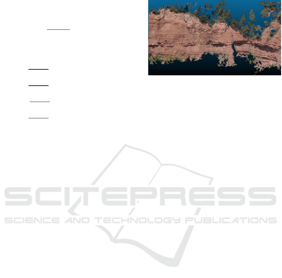
The 3D point cloud model obtained has a high
quality, Figure 1. It is dense, homogeneous and has
information of the rocky wall and the vegetation
around and on it. The vegetation covers the top of the
slope with trees, the face of the slope is covered in
some parts by shrubs, and where it finishes the ground
is covered by grass some bushes and small trees.
One option that could have been used would be
the tools implemented in Agisoft Metashape to
eliminate vegetation and to achieve a model free of
vegetation. That can be compared with the one
obtained with our approach. But it was not possible
because the software does not allow us to customize
these filtering tools and part of the vegetation
remains.
Figure 1: 3D point cloud model obtaining by
photogrammetry.
2.2 Image Classification
The image classification was carried out using the
commercial software ENVI.
In the case of working with the original images
we have chosen a supervised classification with both
visible bands, RGB, and six bands, RGB+HSV.
The first step was to build the RGB+HSV images.
After that, the regions of interest (ROI’s) were chosen
to train the classification model. We considered three
different set of classes:
5 classes: sky, vegetation, shadow in
vegetation, rocky wall, shadow in rocky wall.
4 classes: sky, shrubs and grass, trees, rocky
wall.
3 classes: sky, vegetation, rocky wall.
The three classifications were applied on the two
images sets: RGB channels, and RGB+HSV.
The image classification was made with two
common methods (Richards, 2013), the Euclidean
minimum distance and the Maximum Likelihood
Estimation (MLE). After the analysis of the results of
the classification and the confusion matrix, the first
one was discarded and the process was continued
using only with MLE. Whilst the general accuracy
with MLE is approximately 98% for all the sets, it
was roughly 85% using the minimum distance
method.
2.2.1 Results
The results obtained for all the images set and all the
classification groups are satisfactory for both RGB
and RGB+HSV. However, we can highlight a slight
improvement when the number of channels is
increased.
GISTAM 2021 - 7th International Conference on Geographical Information Systems Theory, Applications and Management
100
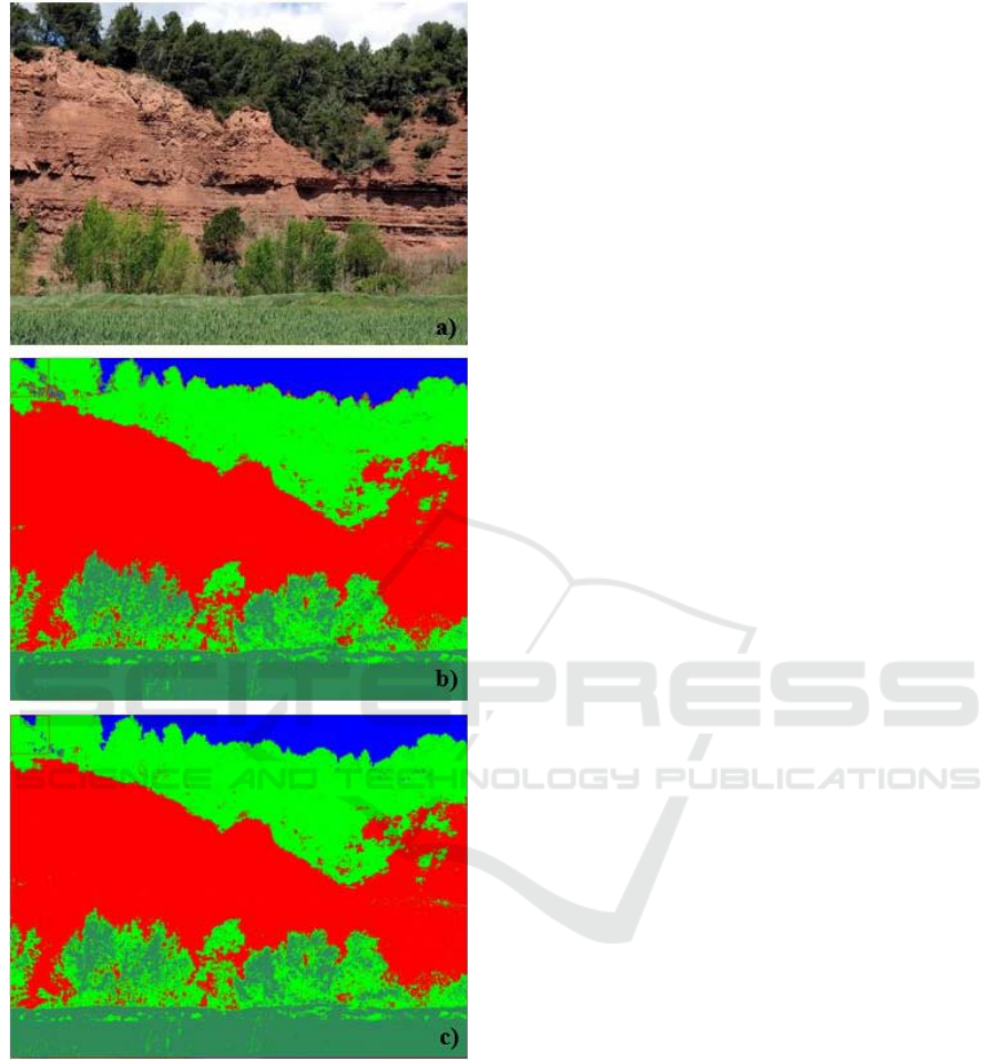
Figure 2: Maximum Likelihood Estimation classification in
4 classes results: a) original RGB image, b) RGB channels,
c) RGB+HSV channels.
Figure 2 shows the classification results using
four classes. The upper image is the original image,
in the centre we locate the classification with an RGB
image, Figure 2. b). It can be seen that the boundary
between classes is less defined than in Figure 2.c),
which uses both RGB+HSV channels, mainly
between the sky and trees class.
With regards the general results, in all the cases
the use of RGB+HSV images allows to achieve a
slight improvement, of less than 1%, in the overall
accuracy compared to the RGB-only analysis.
However, this improvement is more pronounced in
the vegetation classification, overall in the shrubs and
grass class, when the number of classes considered is
decreased.
Using three, four, or five classes the behaviour is
similar. The accuracy in the omission decreased when
the additional information of the hue is considered in
the classification.
2.3 Point Cloud Segmentation
Working with point clouds, the segmentation has
been carried out considering three parameters: the
colour indexes VVI, the ExG, and finally with the
coordinates of the colour space HSV.
We have implemented in Python language a
program to read the point cloud and calculated the
two indices and the HSV coordinates.
For the VVI calculation the values for the vector
of the reference green colour RGB
0
, eq (1), are
R
0
=60.0, G
0
=70.0 and B
0
=30.0, and the weight
component w= 1.
The problem in this index is to set the reference
values, since they depend on the image and the
characteristics of the zone.
After the colour space change, it was checked that
the hue coordinate, such as the eq. (5) shows its value
range from 0º to 360º, is the one that provides most
useful information for the segmentation. For this
reason, the value and the saturation coordinates have
not been considered in the classification.
Analysing the distribution of frequencies for the
VVI, ExG and H values it can been observed that they
follow a bimodal curve, Figure 3, and the minimum
between then could be established as the threshold to
segment the point cloud. In this way, during filtering
using the ExG index we have considered vegetation
points with ExG > -0.02, Figure 3.
In all the areas classified the hue coordinate shows
a similar behaviour. The higher values, more than
300º, are located in areas covered by shadows, Figure
4. Therefore, we have to considerer the minimum
between the distributions and then the tile to segment
correctly the point cloud.
Vegetation Filtering using Colour for Monitoring Applications from Photogrammetric Data
101

Figure 3: Bimodal curve from the ExG values.
It has been considered that if we have more
classes than bare ground and vegetation this approach
should be reconsidered to find the thresholds.
Figure 4: Bimodal curve from the H values.
The result after executing the program are for each
index two files, one with the vegetation and other
with the bare ground and rocks, i.e. six files are
obtaining.
2.3.1 Results
Figure 5 shows the results of the classification using
the different indices. In all the images the bare ground
has been represented in grey colour. In a qualitative
analysis, as the images shown the best results are
obtained using the ExG index and the hue value,
Figures 5.b) and c) respectively. The worst results are
gotten with the VVI, which shows as vegetation the
shadow areas.
The Figure 5.d) shows in red the shadow areas
where the H value reaches more than 300º. These
extreme values are represented in the tile of the
histogram as we have mentioned previously.
Figure 5: Results after the classification, a) VVI, b) ExG, c)
Hue values eliminating the tile of the distribution and d)
Hue values with the values higher 300º.
A common problem is due to the lack or existence
of misleading information in the treetops. Since the
branches and leaves are not in the same position in all
the images, by the wind effect, they appear in the 3D
model without colour. Therefore, they cannot be
classified using this characteristic.
Moreover, we have classified the point cloud with
Canupo (Brodu & Lague, n.d.), Figure 6, to test the
GISTAM 2021 - 7th International Conference on Geographical Information Systems Theory, Applications and Management
102
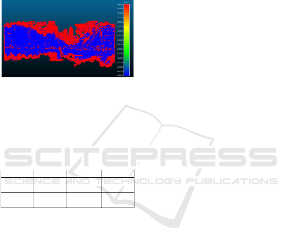
influence of the use of geometry components in the
result improvement. In a qualitative comparison with
the results, Figure 5, we can see that there are zones
of bare ground classified as vegetation, such as with
the use of VVI.
Figure 6: Results of classification with Canupo, in red
vegetation and blue bare ground.
Table 1 shows a quantitative comparison of the
filter methods: the number of points classify as bare
ground, vegetation, and percentages of filtered
vegetation points by the three indices. The values of
shadows, the tile in the histogram, are not considered
for the hue.
Table 1: Number of points in the filtered point clouds and
the percentage of the correct vegetation filtered.
Groun
d
Ve
g
etation % filtere
d
VVI 3.39M 1.09M 75.8
ExG 3.40M 1.08M 94.8
Hue 3.40M 1.08M 95.3
Canupo 3.06M 1.58M 62.5
The ExG and H classify almost the whole of the
vegetation points. The percentages of commission are
around 2% and 1.5%, respectively, mainly in the
zones of shadow boundary between the ground and
the bushes. This percentage increases dramatically
when we use Canupo.
In other study areas, where the point cloud was
obtained by TLS with only an internal camera, the
results were worst. Mainly, due to the illumination is
not the best, since the sensor takes photographs in an
automatic way with the same parameter for all of
them.
3 DISCUSION AND FINAL
REMARKS
The filters that were used in this study have the
advantage that are easy to implement. Moreover, the
results let us be optimistic in the vegetation filtering
using only colour information though indices or the
values of Hue derived directly from the visible bands.
We have used images taken with a common
camera, therefore the cost of this sensor is cheaper
than other methods. The use of the NIR band could
improve the results but these cameras are more
expensive if the resolution want to be kept.
The ExG index and the H value in the case of point
clouds allows us a good classification in the areas
where the model have been built correctly. In
elements that appear moved between a photographs
and other such as the leaves moved by the wind, the
colour is not assigned to the point in the point cloud
and therefore cannot be classify by this characteristic.
Whether the classification is made directly on the
images the use of the H value added to the RGB bands
allow to improve the results without increasing
significantly the time of computation.
4 CONCLUSIONS
In the monitoring of rocky massif to prevent rockfalls
is not possible to use LiDAR due to the verticality of
the walls. Therefore, we cannot take advantage of the
use of several signal echoes to classify vegetation.
Multi-spectral cameras are an alternative. However,
their high cost makes us to discard them.
In this paper, we have proposed the use of the
RGB channels for two purposes, on one hand to
obtain vegetation indices based on the visible
channels and, on the other hand to add additional
HSV channels to the images and point cloud
previously to classify them.
The results show that the combination of the RGB
bands allows us to filter vegetation with methods of
simple application using a common camera, therefore
it is cheaper than other options.
The image classification using as additional band
the Hue value derived of the RGB improves the
result. This improvement is higher when the number
the classes decrease.
The point cloud classification has good results
using the ExG and H values. The success of VVI
index is conditioned by the reference vector, whose
adjustment depends on the scene to classify and it is
more influenced by colour variations and shadows.
However, shadows and boundary zones are where
more misleading classification exist, in all cases.
Vegetation Filtering using Colour for Monitoring Applications from Photogrammetric Data
103

ACKNOWLEDGEMENTS
This study was supported by the National Research
Project "Advances in rockfall quantitative risk
analysis (QRA) incorporating developments in
geomatics (GeoRisk)” funded by the Spanish
Ministry of Economy and Competitiveness, and co-
funded by the Agencia Estatal de Investigación
(AEI) on the framework of the State Plan of
Scientific-Technical Research and Innovation with
reference code PID2019-103974RB-I00/AEI/
10.13039/501100011033.
REFERENCES
Barbarella, M., Fiani, M., & Lugli, A. (2015). Landslide
Monitoring Using Multitemporal Terrestrial Laser
Scanning for Ground Displacement Analysis.
Geomatics, Natural Hazards and Risk 6(5–7):398–418.
Becker, C., Häni, N., Rosinskaya, E., D’Angelo, E., &
Strecha., C. (2017). Classification of aerial
photogrammetric 3D point clouds. ISPRS Annals of the
Photogrammetry, Remote Sensing and Spatial
Information Sciences 4(1W1):3–10.
Brodu, N., & Lague, D. (n.d.). 3D Terrestrial lidar data
classification of complex natural scenes using a multi-
scale dimensionality criterion : applications in
geomorphology .
Dolan, A. M., & Thompson, R. M. (2014). Integration of
drones into domestic airspace: Selected legal issues.
Domestic Drones: Elements and Considerations for the
U.S., 1–41.
Eisenbeiβ, H., Lambers, K., & Sauerbier, M. (2005).
Photogrammetric recording of the archaeological site of
Pinchango Alto (Palpa, Peru) using a mini helicopter
(UAV). In A. Figueiredo (Ed.), Annual Conference on
Computer Applications and Quantitative Methods in
Archaeology CAA (Issue March 2005, pp. 21–24).
http://www.photogrammetry.ethz.ch/general/persons/k
arsten/paper/eisenbeiss_et_al_2007.pdf
Jaboyedoff, M., Oppikofer, T., Abellán, A., Derron, M. H.,
Loye, A., Metzger, R., & Pedrazzini, A. (2012). Use of
LIDAR in landslide investigations: A review. Natural
Hazards, 61(1), 5–28. https://doi.org/10.1007/s11069-
010-9634-2
Kamps, M. T., Bouten, W., & Seijmonsbergen, A. C.
(2017). LiDAR and orthophoto synergy to optimize
object-based landscape change: Analysis of an active
landslide. Remote Sensing, 9(8).
https://doi.org/10.3390/rs9080805
Loesdau, M., Chabrier, S., & Gabillon, A. (2014). Hue and
Saturation in the RGB Color Space BT - Image and
Signal Processing. Springer International Publishing
Switzerland 2014, 203–212.
Niethammer, U., James, M. R., Rothmund, S., Travelletti,
J., & Joswig, M. (2012). UAV-based remote sensing of
the Super-Sauze landslide: Evaluation and results.
Engineering Geology, 128, 2–11.
https://doi.org/10.1016/j.enggeo.2011.03.012
Núñez-Andrés, M. A., Buill, F., Hürlimann, M., & Abancó,
C. (2019). Multi-temporal analysis of morphologic
changes applying geomatic techniques. 70 years of
torrential activity in the Rebaixader catchment (Central
pyrenees). Geomatics, Natural Hazards and Risk,
10(1), 314–335.
https://doi.org/10.1080/19475705.2018.1523235
Ponti, M.P. (2013). Segmentation of Low-Cost Remote
Sensing Images Combining Vegetation Indices and
Mean Shift. IEEE Geoscience and Remote Sensing
Letters 10(1):67–70.Varnes, DJ. 1978. “Transportation
Research Board Special Report: Slope Movement
Types and Processes.” Pp. 11–33 in Landslides,
analysis and control., edited by K. R. ( Schuster RL.
Washington D.C: National Academy of Sciences.
Roncella, R., Forlani, G., Fornari, M., & Diotri, F. (2014).
Landslide monitoring by fixed-base terrestrial stereo-
photogrammetry, ISPRS Ann. Photogramm. Remote
Sens. Spatial Inf. Sci., II-5, 297–304,
https://doi.org/10.5194/isprsannals-II-5-297-2014,
2014.
Richards, J. A. (2013). Remote sensing digital image
analysis: An introduction. (Vol. 9783642300622, pp.
1–494). Springer-Verlag Berlin Heidelberg.
https://doi.org/10.1007/978-3-642-30062-2
Stöcker, C., Bennett, R., Nex, F., Gerke, M., &
Zevenbergen, J. (2017). Review of the current state of
UAV regulations. Remote Sensing, 9(5), 33–35.
https://doi.org/10.3390/rs9050459
Travelletti, J., Delacourt, C., Allemand, P., Malet, J. P.,
Schmittbuhl, J., Toussaint, R., & Bastard, M. (2012).
Correlation of multi-temporal ground-based optical
images for landslide monitoring: Application, potential
and limitations. ISPRS Journal of Photogrammetry and
Remote Sensing, 70, 39–55.
https://doi.org/10.1016/j.isprsjprs.2012.03.007
Tziavou, O., Pytharouli, S., & Souter, J. (2018). Unmanned
Aerial Vehicle (UAV) based mapping in engineering
geological surveys: Considerations for optimum
results. Engineering Geology, 232(June 2017), 12–21.
https://doi.org/10.1016/j.enggeo.2017.11.004
Varnes, D. (1978). Transportation Research Board Special
Report: slope movement types and processes. In K. R.
( Schuster RL (Ed.), Landslides, analysis and control.
(pp. 11–33). National Academy of Sciences.
Xue, J., & Su, B. (2017). Significant remote sensing
vegetation indices: A review of developments and
applications. Journal of Sensors, 2017.
https://doi.org/10.1155/2017/1353691
Yadav, M., Lohani, B., Singh, A.K., & Husain., A. (2016).
“Identification of Pole-like Structures from Mobile
Lidar Data of Complex Road Environment.”
International Journal of Remote Sensing 37(20):4748–
77.
GISTAM 2021 - 7th International Conference on Geographical Information Systems Theory, Applications and Management
104
