
Subcycle-based Neural Network Algorithms for Turning Movement
Count Prediction
Yashaswi Karnati
a
, Rahul Sengupta
b
, Anand Rangarajan
c
and Sanjay Ranka
d
Department of Computer and Information Science & Engineering, University of Florida, Gainesville, FL, U.S.A.
Keywords:
Deep Learning, Intelligent Transportation, Machine Learning, Neural Networks, Turning Movement Count
Prediction.
Abstract:
Predicting intersection turning movements is an important task for urban traffic analysis, planning, and signal
control. However, traffic flow dynamics in the vicinity of urban arterial intersections is a complex and nonlin-
ear phenomenon influenced by factors such as signal timing plan, road geometry, driver behaviors, queuing,
etc. Most current methods focus on predicting turning movement counts using data at coarser aggregations
in the order of minutes or above. Important details such as platoon movements may be lost at such coarse
resolutions. In this work, we propose machine learning approaches to imputing turning movement counts at
intersections using data at subcycle resolutions, from 5 seconds to 375 seconds. In particular, we show that
deep neural networks are capable of directly learning an abstract representation of intersection traffic dynam-
ics using detector actuation waveforms and signal state information. We generate a large dataset of 30 million
cycles by approximately replicating real-world traffic arrival patterns from archived loop detector data in a
microscopic traffic simulator. We extensively evaluate our models and show that our models predict turning
movement counts with greater accuracy when higher resolution data are provided.
1 INTRODUCTION
Turn movement counts (TMCs) are used for a wide
variety of applications related to intersection analy-
ses, intersection design, and transport planning. Re-
cently, several advances in traffic control technolo-
gies and applications are driving additional needs for
continuous, real-time, quality TMC data. These tech-
nologies include:
1. Adaptive control technologies: These systems dy-
namically change the signal phasing pattern lo-
cally at an intersection based on traffic demand.
2. Regional Integrated Corridor Management Sys-
tem (R-ICMS): This system will perform a meso-
scopic simulation of the network using TMCs to
validate the improvement to the network if a di-
version route response plan is implemented or an
optimized set of signal timing plans is deployed.
These applications have introduced additional
traffic data needs beyond what has been provided with
a
https://orcid.org/0000-0002-2512-1250
b
https://orcid.org/0000-0001-9793-5176
c
https://orcid.org/0000-0001-8695-8436
d
https://orcid.org/0000-0003-4886-1988
the traditional TMC data collection efforts, as fol-
lows:
1. Temporal coverage: The data need to be provided
for intersections continuously, not just for a sam-
pling of time for a few hours or days.
2. Spatial coverage: The data need to be provided
for intersections throughout an entire corridor or
network in order to support a regional application.
3. Cost effective: The data need to be able to be col-
lected in a cost-effective manner, which requires
the use of technology instead of manual counts.
This derives from the need for temporal and spa-
tial coverage.
4. Real-time: The data need to be available in real-
time for use by real-time operations.
5. Higher granularity: The TMC data need to be ac-
curate for several cycles to a few hours.
The traditional method of using a human to ob-
tain this information manually is very time consuming
and monotonous. Although approach volumes can be
easily derived from the loop detectors, they only give
information on how many vehicles are entering the in-
tersection and not the TMCs. The focus of this work
Karnati, Y., Sengupta, R., Rangarajan, A. and Ranka, S.
Subcycle-based Neural Network Algorithms for Turning Movement Count Prediction.
DOI: 10.5220/0010501407350744
In Proceedings of the 7th International Conference on Vehicle Technology and Intelligent Transport Systems (VEHITS 2021), pages 735-744
ISBN: 978-989-758-513-5
Copyright
c
2021 by SCITEPRESS – Science and Technology Publications, Lda. All rights reserved
735

in on accurately and efficiently deriving TMCs using
loop detector data by utilizing machine learning tech-
niques.
So far, intersection systems have only given data
at coarse levels of granularity (for example, traffic
movement counts by hour) limiting their use. The
recent advent of automated traffic signal performance
measures (ATSPM) systems provides this information
and signal timing information at a decisecond level.
Availability of this information along with the avail-
ability of cheap GPU-based computing and deep neu-
ral network algorithms has opened up the possibility
of modeling traffic behavior at the subcycle level and
is the focus of this paper.
The rest of the document is described as follows.
Section 2 presents the related work of different tech-
niques used for turning movement counts prediction.
Section 3 describes how we preprocess raw data and
generate synthetic datasets from real-world controller
log data using SUMO (Lopez et al., 2018). In sec-
tion 4, we present the machine learning models devel-
oped for predicting turning movement counts and sev-
eral experimental results. Conclusions are provided in
Section 5.
Our contributions can be summarized as follows:
• We show that using detector waveforms instead
of aggregated traffic volumes leads to better accu-
racy for turning movement counts prediction. Our
neural network models perform well both under
unsaturated and oversaturated conditions.
• We have developed neural network models for
predicting turning movement counts for an inter-
section, given information from stop bar detectors
and advance detectors of the intersection and ad-
vance detectors of upstream intersections. Our ap-
proach uses a novel modular neural network archi-
tecture for predicting turning movement counts.
By using a common weight matrix for all four di-
rections in the first hidden layer of the network,
the size of this network is much smaller than a typ-
ical feed-forward network, thereby reducing the
uncertainty in predictions.
• We have developed a system for generating syn-
thetic datasets with traffic distributions close to
real world. We used detector controller logs from
300 intersections in Orlando to construct inflow
waveforms and fed them into SUMO to run simu-
lations.
2 RELATED WORK
In this section, we summarize the existing literature
on turning movement counts prediction. We broadly
categorize the existing literature and summarize each
category.
2.1 Flow-based Methods
Some studies, (Chen et al., 2012; P. T. Martin, 1992;
Wu and Thnay, 2001; Xu et al., 2013), have used
mathematical techniques like linear programming to
impute turning movement counts which balances in-
flow, outflow of traffic with some constraints. By
modelling the flow with some constraints as linear
equations, we can solve for every unknown movement
if we have enough equations. To calculate westbound
through volume at intersection i, the following equa-
tion can be used.
W BT
t
i
= −NBL
t
i
− SBR
t
i
+W BR
t+δt
j
+W BL
t+δt
j
+W BT
t+δt
j
− δ
t
i j
(1)
where
WBT: westbound through
NBL: northbound left
SBR: southbound right
WBR: westbound right
WBL: westbound left
t: time interval t
i,j: intersections number
∆t time taken to travel between i,j
δ
t+∆t
i j
: additional trips generated between inter-
sections i, j during time interval ∆t.
In the equation, ∆t is assumed to be zero if the dis-
tance between the two intersections is small because
the volume fluctuations would be significantly low.
Also, δ
i j
can be assumed to be zero if there are no
trips generated between these two intersections.
Linear programming-based approaches
(P. T. Martin, 1992) have been used to compute
turning movement counts using flows. This approach
requires measurements like detector flow, weight
given to each link, and constraints on flow for each
link. A system of linear equations is modelled with
the above constraints and information. This system of
equations is solved to get turning movement counts.
Methods based on origin-destination (O-D) ma-
trices to compute turning movement counts (Wu and
Thnay, 2001) uses already observed O-D matrices to
predict future O-D matrices. They use a travel de-
mand model, the Furness Method, and then use the
equilibrium principle to assign future O-D matrices
to the network.
iMLTrans 2021 - Special Session on Intelligent Mobility, Logistics and Transport
736
A
S
A
Stopbar detector
Advance detector
O
Outflow detector
O
S
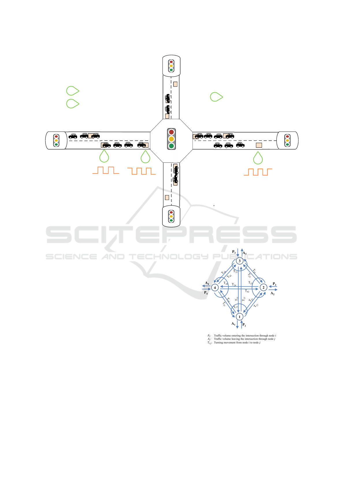
Figure 1: Diagram showing a typical intersection. Arrival/departure waveforms are observed at stop bar (S) and advance (A)
detectors.
The path flow estimator (Chen et al., 2012) com-
putes complete link flows along with turn movement
counts when some traffic counts at selected intersec-
tions are known. The proposed algorithm iterates over
entropy and equilibrium terms to obtain the final solu-
tion. The first term, entropy, distributes trips to multi-
ple paths. The second term, equilibrium, makes those
trips cluster together on minimum cost paths. The al-
gorithm has an outer loop to iteratively generate paths
to the working path set as needed to replicate the ob-
served link counts, turning movement counts, and se-
lected prior O-D flows. The claim is that the method
has advantages because of the single level convex
programming formulation, when compared to other
bilevel programming approaches.
2.2 Neural Network-based Approaches
These methods (Ghanim and Shaaban, 2019) use only
approach volumes to predict corresponding turning
movement counts. Figure 2 shows how a four-leg in-
tersection is represented as a node where the number
of vehicles leaving the node i is P
i
: P
i
=
∑
4
j=1
T
i j
. The
turning movement counts between node i and node j
are the number of trips from i to j. So, when a vehicle
Figure 2: Representation of signalized intersection pro-
posed in (Ghanim and Shaaban, 2019).
is approaching an intersection, they have four possible
turns: left, through, right, and U-turn. For the four ap-
proaches, there are 16 possible movements. For inter-
section j, the number of vehicles attracted to it is A
j
:
A
j
=
∑
4
i=1
T
i j
; this is the sum of all the trips with des-
tination j. So 16 different turning movement counts
should be modelled with the help of known values.
Each T
i j
is modelled as a function of P
i
and A
j
. (Lv
Subcycle-based Neural Network Algorithms for Turning Movement Count Prediction
737

et al., 2015) uses a stacked autoencoder model to pre-
dict traffic flow. An autoencoder is a neural network
that tries to reproduce its input. It acts as an iden-
tity function. It tends to learn features that form a
good representation of its input. Stacked autoencoder
models are created by stacking autoencoders in a hi-
erarchical way. The generic traffic flow features are
modelled with a stacked autoencoder model. They
also take into account spatial and temporal correla-
tions. They use a logistic regression layer as the top
layer for supervised traffic prediction.
2.3 Other Approaches
Approaches such as the genetic algorithm-based
framework (Pengpeng Jiao, 2005) are also used to ob-
tain a dynamic relation between turning movement
proportions and traffic counts at an intersection at
each time step. The proposed objective function min-
imizes the sum of absolute differences between ob-
served and predicted traffic counts. The objective
function is made to converge using a revised pa-
rameter optimization model. Then, they finally pro-
pose a genetic algorithm to impute turning movement
counts.
The current state of research is lacking in several
aspects. The datasets used are often small and don’t
represent a wide variety of traffic scenarios that may
occur. Current methods use data aggregated at res-
olutions in the order of minutes and above and thus
miss important details that may be found in more fine-
grained data.
Our approach is different for two reasons:
1. Large number of samples collected using a realis-
tic simulation framework
2. Results show that using more fine-grained data
results in better accuracy for turning movement
count prediction.
3 DATASETS AND
PREPROCESSING
In this section, we describe the data preprocessing and
dataset generation pipeline. We find that the present
datasets on turning movement counts are inadequate
for our needs. Hence, we use the SUMO microscopic
simulator programmed with real-world traffic flows
and signal plans to generate our dataset. Specifically,
using SUMO helps us in the following ways:
• Datasets are often aggregated at 30-minute inter-
vals, which is too coarse for our needs. SUMO
allows us to generate data at 1-second resolution.
• Actual (ground truth ) turning movement counts
are not readily available nor is there a straightfor-
ward way of using controller log data for imputing
them. SUMO logs allow us to get ground-truth
turning movement counts.
• Another challenge is that we do not have a detec-
tor channel to acquire phase mappings for most of
the intersections. So, the information from con-
troller logs cannot be used in a structured manner
(we do not know whether a detector belongs to a
major or minor street or is advance or at a stop
bar). Because we place the detectors in SUMO,
we know their locations and functions precisely.
One important aspect of simulations is modeling
the demand to be as realistic as possible. Program-
ming random flows or using coarse origin-destination
matrices for generating flows may lead to unrealis-
tic traffic distributions. The real-world dataset we use
to program our simulation consists of controller log
data from 329 signalized intersections in Seminole
County, Greater Orlando Metropolitan Area. For traf-
fic flows, we use loop detector waveform data from
advance detectors of these intersections and regener-
ate them in our simulations. We create a huge syn-
thetic dataset of 30 million cycles, with traffic dis-
tributions similar to those observed in the real world.
(The process is described in 3.2.)
3.1 Recorded High Resolution Loop
Detector Data
High-resolution loop detector data and signal tim-
ing data captured by ATSPM (Day et al., 2014) is
valuable for characterizing the performance of in-
tersections using various Measures of Effectiveness
(MoEs). Induction loop detectors attached to the in-
tersection collect data at 10 Hz, indicating whether a
vehicle passed over or not. Signal behavior is also
captured. These data allow traffic engineers to ana-
lyze the performance of traffic intersections and im-
prove safety and efficiency while cutting costs and
congestion.
Table 1 shows a sample of high resolution data.
The data consist of the following attributes:
1. SignalID: Intersection identifier
2. Timestamp: Time at which event was logged (de-
cisecond resolution)
3. EventCode: What event at the signal was captured
4. EventParam: What was the value of the event or
attribute at that timestamp.
These data also come with metadata which de-
scribe what different event codes and event param-
iMLTrans 2021 - Special Session on Intelligent Mobility, Logistics and Transport
738

Table 1: Raw event logs from signal controllers. Most mod-
ern controllers generate these data at a frequency of 10 Hz.
SignalID Timestamp EventCode EventParam
1490
2018-08-01
00:00:00.000100
82 3
1490
2018-08-01
00:00:00.000300
82 8
1490
2018-08-01
00:00:00.000300
0 2
1490
2018-08-01
00:00:00.000300
0 6
1490
2018-08-01
00:00:00.000300
46 1
1490
2018-08-01
00:00:00.000300
46 2
1490
2018-08-01
00:00:00.000300
46 3
eters indicate, for example, event code 81 indicates a
vehicle departure, event code 2 indicates start of green
phase, etc. The event parameter identifies the partic-
ular detector channel or phase in which the event was
captured.
3.2 Data Generation
In order to model an intersection, we need a large
dataset to train our models. While several real-world
datasets exist (Wang et al., 2019), they are of limited
utility for our task because they do not model inter-
sections under diverse traffic and signal timing condi-
tions.
Along with diverse but realistic traffic flows, we
also need to program realistic traffic signal plans. In
the real world, it is highly unlikely that a traffic au-
thority would implement undesirable signal timing
schemes for gathering data because that would have
adverse real-world consequences. On the other hand,
microscopic simulators offer us the flexibility of im-
plementing undesirable signal timing plans. We study
the Orlando dataset and derive a signal timing plan as
shown in Table 2.
The signal timing plan for the intersection is an
actuated signal timing plan with minimum and maxi-
mum times, as shown in Table 2.
A yellow time of 5 seconds follows each phase.
Thus, this leads to a theoretical minimum signal cycle
length of 60 seconds and a maximum length of 180
seconds. This maximum is chosen with consideration
of acceptable pedestrian wait times.
We use a three-stage approach for generating sim-
Table 2: Actuated Signal Timing Plan Details.
Traffic Min Green Max Green
Movement Time (seconds) Time (seconds)
Corridor Through/Right 20 70
Side-Through/Right 10 30
Corridor Left 10 30
Side Left 10 30
ulated data:
1. Generate a realistic intersection configuration in
SUMO
2. Derive traffic waveforms from real data
3. Run parallel simulations using waveforms from
step-2 and intersection configuration in step-1.
3.3 Intersection Configuration
Our simulation consists of a one-intersection sce-
nario with four approaches, based on standard
NEMA (National Electrical Manufacturing Associa-
tion) (US Department of Transportation, 2008) phas-
ing. It consists of four through or right movements
and four left-turn movements, one of each movement
for the four approaches. Most urban arterials have an
exclusive left-turn buffer at each approach to cater to
the left-turning traffic. This prevents the left-turning
traffic from blocking the through and right traffic until
the buffer is filled.
Each approach is initially a single lane which
fans out into a through-lane and an exclusive left-turn
buffer. The left-turn buffers extend 60 meters and can
hold 6-7 vehicles. There are two stop bar detectors
per approach, one each for through/right and left turn
lanes. There is one advance detector 90 meters from
the intersection, just beyond the end of the left-turn
buffer. This minimal configuration captures all the
eight turn movements possible. Multiple lanes for
each movement group can be handled by (a) aggre-
gating detector counts per movement group and (b)
training multiple models, one for each intersection ge-
ometry of interest. In this study, we only focus on the
most general and minimal configuration.
In order to gather downstream data, we place gat-
ing traffic signals that mimic a downstream intersec-
tion 800 meters from the main intersection. They
are simple one-phase signals without any side streets.
Adding fully-fledged intersections with coherent real-
world flows would have been computationally expen-
sive and will be included in a follow-up extension to
this work. There are four such gating signals, one
along each of the four outbound directions.
Subcycle-based Neural Network Algorithms for Turning Movement Count Prediction
739

3.4 Input Traffic Generation
Archived controller logs are used to construct inflow
waveforms along all four directions. These wave-
forms are in turn used to inject vehicles into SUMO
from four directions with an adaptive signal timing
control. This way, we generate datasets whose inflow
and outflow distributions are close to what we observe
in the real world. For this, we used six months of con-
troller logs from 90 intersections in the City of Or-
lando.
Thus, the main flow along corridor through and
right directions will be between two to eight times the
flow along the other streets. These ratios are based
on the observed traffic flows in the recorded Orlando
dataset.
We use advance detector logs from the Orlando
dataset to generate vehicle flows at a 1-second res-
olution. We randomly sample flow patterns ob-
served at these two detectors for the straight and side
streets and ensure that they fall between the above-
mentioned volume flow constraints. We program
these arrival patterns into SUMO. These patterns are
further shaped by the gating signals at the start of the
four incoming approaches. This ensures variable pla-
tooning of volumes based on real-world data.
3.5 Parallel Dataset Generation
The data generation process makes use of the multi-
processing environment. At any instant, several simu-
lations will be running in parallel: each thread runs a
simulation, processes the logs, and dumps the dataset
into the file system.
Each simulation generates logs which have infor-
mation of every time step of the simulation. These
logs are processed, and the following information is
stored:
• Waveforms at all the stop bar and advance detec-
tors for all the approaches
• Waveforms at all the advance detectors of nearby
intersections
• Signal timing information
• Turn movement counts for all the possible move-
ments.
Within a simulation, after an initial simulation
warm-up of 600 seconds, logs are extracted in win-
dows of 1,000 seconds. These usually contain 8-9
complete cycles on average. Thus, each data exem-
plar consists of a set of waveforms of different sig-
nals and detectors, queue lengths, and turn movement
counts for a window of 1,000 seconds (T = 200), ag-
gregated at 5-second resolution.
A large dataset of 5 million such exemplars is thus
generated, accounting for 30 million traffic cycles of
simulation. The dataset is then split for training and
testing in the ratio of 70:30.
The creation of such a vast dataset involved con-
siderable engineering effort. The entire pipeline was
implemented in the Python programming language. A
multiprocessing library was used to run up to 60 par-
allel instances of SUMO and preprocess output XML
logs in batches. Numpy (Harris et al., 2020) and
Dask (Rocklin, 2015) were then used to create vectors
for training and testing. These vectors were stored
in HDF5 format using the H5PY (Collette, 2013) li-
brary.
Implementation, training, and evaluation of the
deep learning models was done using the Py-
Torch (Paszke et al., 2019) library. University of
Florida’s HiPerGator supercomputing resources were
used to train and test multiple models in parallel.
We use this dataset for modelling a universal ap-
proximator for predicting turn movement counts. The
inputs to the model are:
• Detector actuations for all advance detectors (four
detectors)
• Detector actuations at stop bar detectors for
through-right and left buffers (eight detectors)
• Detector actuations at early detectors of nearby in-
tersections (outflow detectors) (four detectors).
The information from these 16 detectors is used to
predict turn movement counts. The detector actua-
tions are aggregated to some level to construct detec-
tor waveforms. These detector waveforms are in turn
used as input to the neural network models.
4 MACHINE LEARNING
MODELS FOR TMC
PREDICTION
The input to the models is detector waveforms (ag-
gregated to some time interval) at stop bar and
advance detectors. The input layer has 16 ×
(numbero f timesteps) neurons, each neuron takes in-
put from one detector and one time point.
The waveforms are represented as 1-D vectors,
each with T components. Here T refers to the length
of time a particular sensor’s data is being considered,
with each component being aggregated at a 5-second
level.
We performed different experiments to analyze
how the following parameters affect the TMC predic-
tion.
iMLTrans 2021 - Special Session on Intelligent Mobility, Logistics and Transport
740
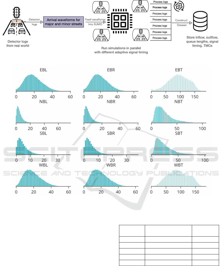
Figure 3: Simulations block diagram.
Figure 4: Turning movement count distributions of the dataset generated by simulation.
• Prediction Window: This defines the time win-
dow for which we predict the TMCs. Based on
our results, we observed that as the size of the pre-
diction window increases, the accuracy for pre-
dicting turning movement counts increases.
• Waveform Aggregation Level: This denotes the
time resolution for each step of the waveform con-
structed from detector actuations. We vary this to
find the optimal value of aggregation level for the
waveform (5 sec, 15 sec, 25 sec, etc.).
We now describe a modular neural network archi-
tecture where input is transformed to the first hidden
layer by sharing a common weight matrix among the
detector waveforms of all the directions. The basic
reasoning is that the detector waveforms (stop bar and
advance) of the four directions would have similar
properties. So, for the feed-forward, network we ana-
Table 3: Table showing MSE on test set for prediction win-
dow of 375 seconds for different waveform aggregation lev-
els.
Predicton
Window
Waveform Aggrega-
tion level
MSE on
Test Set
375 sec 5 sec 0.0002
375 sec 15 sec 0.0005
375 sec 25 sec 0.0002
375 sec 75 sec 0.0004
375 sec 375 sec 0.001
lyze the weights connecting the inputs to first hidden
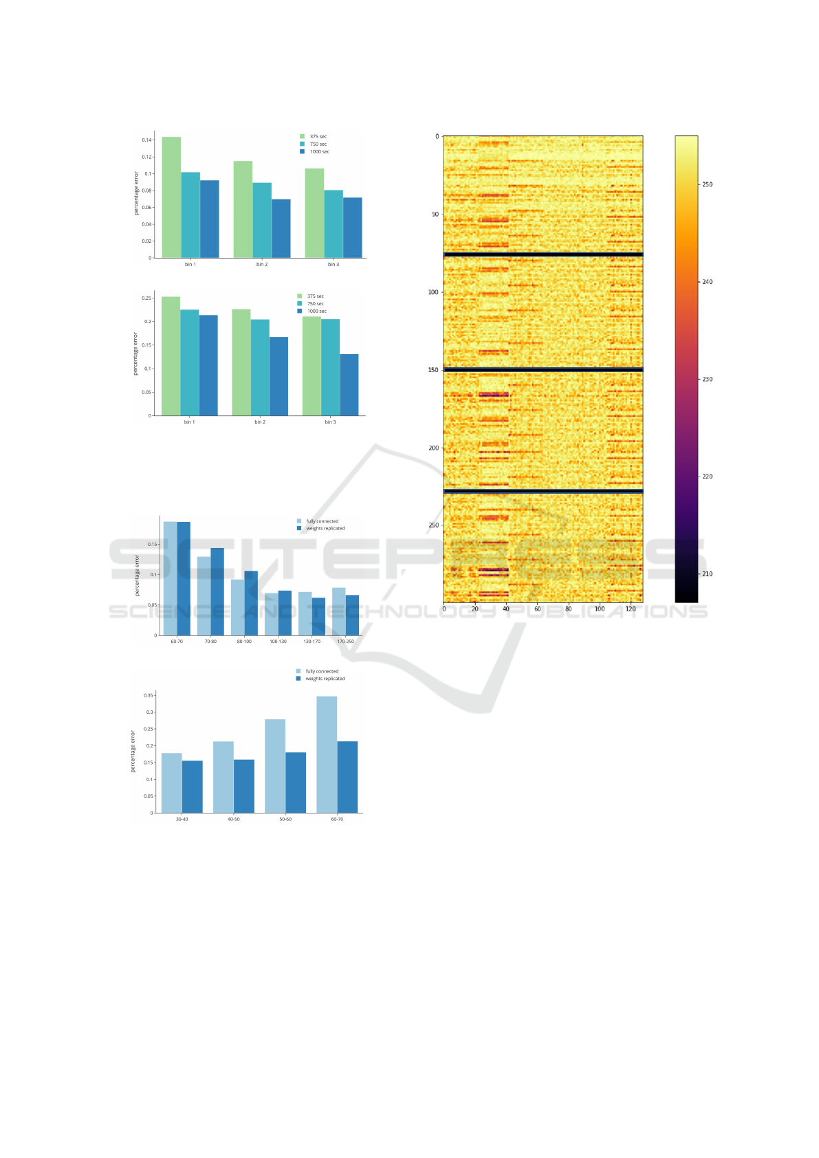
layer. Figure 10 shows the heat map of weights con-
necting the input layer to the first hidden layer of the
feed-forward network. In the plot the absolute value
of weights is taken, multiplied by 100 to highlight the
trends. The red marker in the plot separates the four
Subcycle-based Neural Network Algorithms for Turning Movement Count Prediction
741
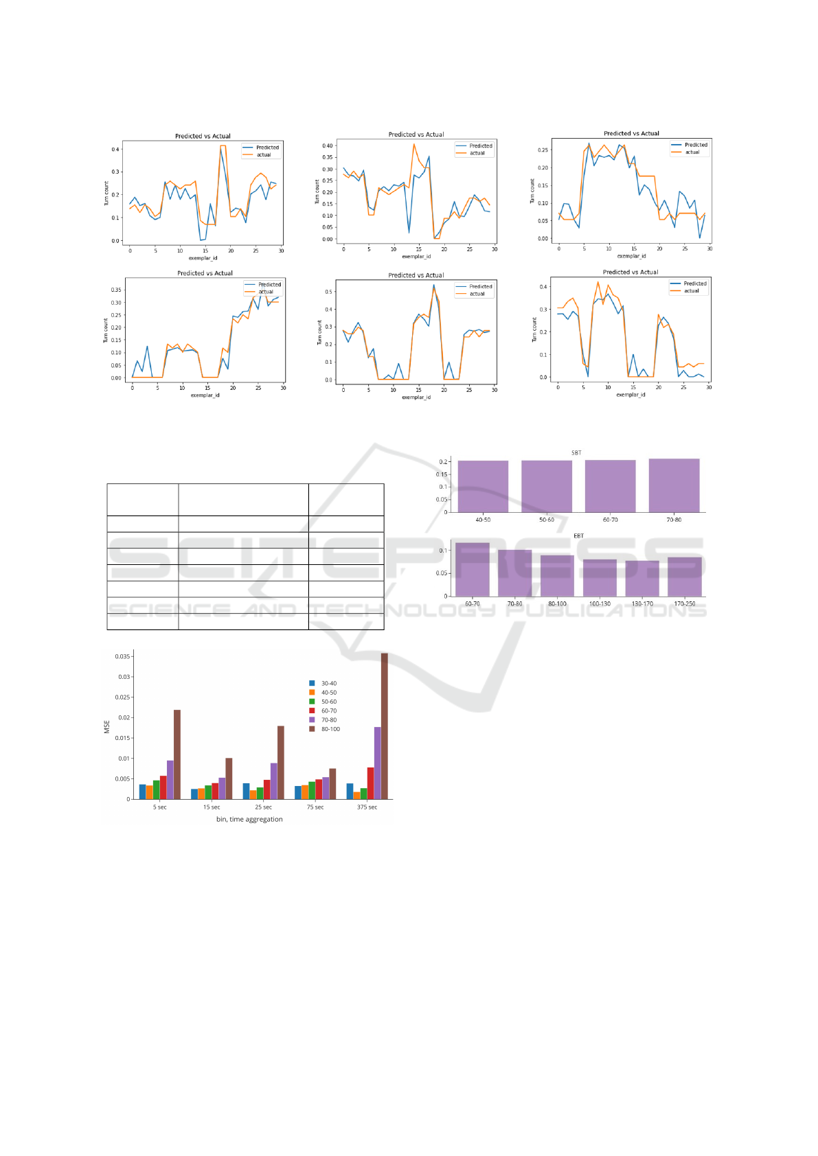
Figure 5: Actual vs. predicted turning movement counts for six different movements using a waveform model. The y-axis
represents particular movements; the x-axis represents random exemplars of the test set.
Table 4: Table showing MSE on test set for different pre-
diction windows.
Prediction
Window
Waveform Aggrega-
tion level
MSE on
Test Set
375 sec 5 sec 0.0002
375 sec 15 sec 0.0005
750 sec 5 sec 0.0005
750 sec 15 sec 0.0006
750 sec 25 sec 0.0005
1000 sec 5 sec 0.0008
1000 sec 20 sec 0.0008
Figure 6: Plot showing MSE for eastbound through traffic
for different bins, comparing different waveform aggrega-
tion levels.
directions, and the detector waveforms on the y-axis
are ordered in correspondence to detectors in this or-
der: east, west, north, and south. We can see from the
plot that the weights connected to detectors on differ-
ent directions look similar.
So to decrease the number of learnable parameters
and get better generalization, a common weight ma-
Figure 7: Plot showing percentage error for comparing dif-
ferent bins. This plot suggests that the model is perform-
ing well irrespective of the saturation level: (a) southbound
through; (b) eastbound through.
trix is used for transforming detector waveforms on
different directions to the first hidden layer. Figure 9
shows the comparison of percentage error for differ-
ent bins comparing a fully connected network with
the modular architecture. We can see that the mod-
ular architecture performs equally well with a lower
number of parameters.
5 CONCLUSIONS
We have developed machine learning models for pre-
dicting turn movement counts for a single intersec-
tion, given information from stop bar and advance de-
tectors. All of these data are available from ground
sensors. Hence, this model can be easily adapted to
practical datasets.
iMLTrans 2021 - Special Session on Intelligent Mobility, Logistics and Transport
742
(a)
(b)
Figure 8: Plot showing percentage error for comparing dif-
ferent prediction windows. This plot suggests that accuracy
increases when predicting for a larger window size: (a) east-
bound through; (b) southbound through.
(a)
(b)
Figure 9: Plot showing comparison between fully con-
nected and weight-sharing model. The weight-sharing
model is comparable or better.
• We developed neural network models for predict-
ing turning movement counts for an intersection,
given information from stop bar and advance de-
tectors of the intersection and advance detectors
of upstream intersections.
Figure 10: Plot showing heat map of weights connecting in-
put layer and first hidden layer.The horizontal black bar sep-
arates the four directions. The ordering of detector wave-
forms along the y-axis is as follows: east, west, north, and
south.
• We developed a system for generating synthetic
datasets with traffic distributions close to real-
world. We used detector controller logs from
300 intersections in Orlando to reconstruct inflow
waveforms and fed them into SUMO for running
simulations.
• We prove that using detector waveforms instead
of aggregated traffic volumes leads to better accu-
racy for predicting turning movement counts.
• The neural network models developed perform
well both under unsaturated and oversaturated
conditions.
• We developed a modular neural network archi-
tecture for predicting turning movement counts.
Instead of using different weight matrices across
four directions (as in general feed-forward net-
works), we use a common weight matrix for all
Subcycle-based Neural Network Algorithms for Turning Movement Count Prediction
743

the four directions in the first hidden layer of
the network. This modular architecture performs
equally well and has fewer learnable parameters
in comparison with a feed-forward network.
ACKNOWLEDGEMENTS
The work was supported in part by NSF CNS
1922782 and by the Florida Department of transporta-
tion (FDOT) District 5. The opinions, findings and
conclusions expressed in this publication are those of
the authors and not necessarily those of FDOT D5.
REFERENCES
Chen, A., Chootinan, P., Ryu, S., Lee, M., and Recker, W.
(2012). An intersection turning movement estimation
procedure based on path flow estimator. Journal of
Advanced Transportation, 46:161 – 176.
Collette, A. (2013). Python and HDF5. O’Reilly.
Day, C. M., Bullock, D. M., Li, H., Remias, S. M., Hainen,
A. M., Freije, R. S., Stevens, A. L., Sturdevant, J. R.,
and Brennan, T. M. (2014). Performance measures for
traffic signal systems: An outcome-oriented approach.
Technical report.
Ghanim, M. S. and Shaaban, K. (2019). Estimating turn-
ing movements at signalized intersections using artifi-
cial neural networks. IEEE Transactions on Intelligent
Transportation Systems, 20(5):1828–1836.
Harris, C. R., Millman, K. J., van der Walt, S. J., Gommers,
R., Virtanen, P., Cournapeau, D., Wieser, E., Taylor,
J., Berg, S., Smith, N. J., Kern, R., Picus, M., Hoyer,
S., van Kerkwijk, M. H., Brett, M., Haldane, A., del
R’ıo, J. F., Wiebe, M., Peterson, P., G’erard-Marchant,
P., Sheppard, K., Reddy, T., Weckesser, W., Abbasi,
H., Gohlke, C., and Oliphant, T. E. (2020). Array pro-
gramming with NumPy. Nature, 585(7825):357–362.
Lopez, P. A., Behrisch, M., Bieker-Walz, L., Erdmann, J.,
Fl
¨
otter
¨
od, Y.-P., Hilbrich, R., L
¨
ucken, L., Rummel, J.,
Wagner, P., and Wießner, E. (2018). Microscopic traf-
fic simulation using sumo. In The 21st IEEE Interna-
tional Conference on Intelligent Transportation Sys-
tems. IEEE.
Lv, Y., Duan, Y., Kang, W., Li, Z., and Wang, F. (2015).
Traffic flow prediction with big data: A deep learn-
ing approach. IEEE Transactions on Intelligent Trans-
portation Systems, 16(2):865–873.
P. T. Martin, M. C. B. (1992). Network programming to
derive turning movements from link flows. In Transp.
Res. Rec., no. 1365, pages 147–154. Transportation
Research Board.
Paszke, A., Gross, S., Massa, F., Lerer, A., Bradbury, J.,
Chanan, G., Killeen, T., Lin, Z., Gimelshein, N.,
Antiga, L., Desmaison, A., Kopf, A., Yang, E., De-
Vito, Z., Raison, M., Tejani, A., Chilamkurthy, S.,
Steiner, B., Fang, L., Bai, J., and Chintala, S. (2019).
PyTorch: An Imperative Style, High-Performance
Deep Learning Library.
Pengpeng Jiao, Huapu Lu, L. Y. (2005). Real-time esti-
mation of turning movement proportions based on ge-
netic algorithm. In Proceedings. 2005 IEEE Intelli-
gent Transportation Systems, 2005., pages 96–101.
Rocklin, M. (2015). Dask: Parallel computation with
blocked algorithms and task scheduling. In Huff,
K. and Bergstra, J., editors, Proceedings of the 14th
Python in Science Conference, pages 130 – 136.
US Department of Transportation, F. H. A. (2008). Traf-
fic signal timing manual. https://ops.fhwa.dot.gov/
publications/fhwahop08024/chapter4.htm. (Accessed
on 03/18/2021).
Wang, Y., Zhang, D., Liu, Y., Dai, B., and Lee, L. H. (2019).
Enhancing transportation systems via deep learning:
A survey. Transportation research part C: emerging
technologies, 99:144–163.
Wu, J. and Thnay, C. (2001). An o-d based method for
estimating link and turning volume based on counts.
In Transp. Res. Rec., no. 1365, pages 865–873. ITE
Dist 6.
Xu, K., Yi, P., Shao, C., and Mao, J. (2013). Development
and testing of an automatic turning movement identi-
fication system at signalized intersections. Journal of
Transportation Technologies, 03:241–246.
iMLTrans 2021 - Special Session on Intelligent Mobility, Logistics and Transport
744
