An Approach to Reduce Network Effects in an Industrial Control

and Edge Computing Scenario

omulo A. L. V. de Omena, Danilo F. S. Santos and Angelo Perkusich

Embedded Systems and Pervasive Computing Lab, Federal University of Campina Grande, 882 Apr

ıgio Veloso St.,

58429-970, Campina Grande, PB, Brazil

Keywords:

IIoT, Industry 4.0, Edge Computing, 5G, Model Predictive Control, AGV.

Abstract:

The cloud-based nature of Industry 4.0 enhances its ﬂexibility and scalability features. To support time-

sensitive and mission-critical applications, whereby low latency and fast response are essential requirements,

usually cloud computing resources should be placed closer to the industry. The Edge Computing concept

combined with next-generation networks, such as 5G, may fulﬁll those requirements. This paper presents an

experimental system setup that combines a Model Predictive Control approach with a compensation strategy

to mitigate network delay and packet loss. The experimental system has two sides, namely, the edge and

the local side. The former executes the controller and connects to the local side through a network. The

latter is attached to the application and has lower computing capabilities. In our setup, the application under

control is a two-wheeled mobile robot, which could act as an Automated Guided Vehicle. We deﬁned two

control objectives, the Point Stabilization, and the Trajectory Tracking, which ran through distinct network

conditions, including delays and packet losses. These control objectives are only validation scenarios of the

proposed approach but could be replaced by a real case path planner. The obtained results suggest that the

approach is valid.

1 INTRODUCTION

Driven by the Internet of Things (IoT) paradigm, the

new era of computing is bringing out the Internet

from the traditional desktop to many objects around

us (Gubbi et al., 2013), based on ubiquitous com-

puting, where smart environments recognize, iden-

tify objects, and retrieves information (Yaqoob et al.,

2017). Applications are spread in several domains,

such as smart homes, healthcare, industrial automa-

tion, agriculture, school, market, and vehicles (Al-

Fuqaha et al., 2015).

The application of IoT in industries covers an area

called the Industrial Internet of Things (IIoT). In an

IIoT system, the industrial “things”, such as sensors,

controllers, actuators, production lines, and equip-

ment, connect to the Internet. They can improve pro-

ductivity, efﬁciency, safety, and intelligence of indus-

trial factories and plants (Xu et al., 2018). Sisinni

et al. (2018) considers the IIoT as a subset of IoT, and

merging IIoT and Cyber-Physical Systems (CPS) re-

sults in the Industry 4.0. An essential feature of IIoT

is the cloud-based nature, making it more ﬂexible and

scalable than conventional industrial systems (Wan

et al., 2016).

To fulﬁll the requirements of mission-critical and

time-sensitive systems, where low latency commu-

nication and fast response are essential, the physi-

cal distance to the cloud computing servers may not

meet those requirements. To deal with cloud com-

puting limitations, the “Edge Computing” concept

has emerged, bringing cloud services closer to de-

vices. It is also known as the “cloud closer to the

ground” (Kaur et al., 2018). In an industrial en-

vironment, edge computing introduces an interme-

diate level, separating the ﬁeld level domain from

cloud-based services. The ﬁeld devices perform tasks

regarded to industrial automation and need to re-

act faster; therefore, latency and reliability are real-

time constraints and requirements of communication

links (Pallasch et al., 2018). In the context of IIoT

and Industry 4.0, edge computing provides high band-

width, low latency, and low jitter, necessary to process

urgent and complex tasks on time. Battery-powered

devices and sensors, restricted in energy consump-

tion, also take advantage of edge computing, as tasks

demanding high processing are transferred to a higher

layer (Aazam et al., 2018).

Qiu et al. (2020) highlights some advantages of

296

V. de Omena, R., Santos, D. and Perkusich, A.

An Approach to Reduce Network Effects in an Industrial Control and Edge Computing Scenario.

DOI: 10.5220/0010496502960303

In Proceedings of the 11th International Conference on Cloud Computing and Services Science (CLOSER 2021), pages 296-303

ISBN: 978-989-758-510-4

the Edge Computing in IIoT: 1) improve system per-

formance by reducing the overall delay of the system;

2) protect data security and privacy, reducing risks of

data leakage; 3) reduce operational costs, as the data

uploading volume to cloud and bandwidth consump-

tion is reduced. Chen et al. (2018) discuss the co-

operation mechanism between Cloud Computing and

Edge Computing. On the one hand, Edge Comput-

ing better supports real-time processing. On the other

hand, Cloud Computing focuses on analyzing big data

and knowledge mining from the data obtained at the

edge, playing an important role in periodic mainte-

nance, decision support, and other tasks that do not

need to be performed in real-time.

When the mobile network provides the edge com-

puting services, it is called Multi-Acess Edge Com-

puting (MEC) (Abbas et al., 2018), which delivers

computing capabilities through the Radio Access Net-

work (RAN), therefore reducing latency and improv-

ing the Quality of Service (QoS) (Kiani and Ansari,

2018). 5G mobile networks are expected to bring net-

works with ultra-low latency and ultra-high reliability

(ULLRC). Thus, the merging of MEC and 5G is ex-

pected to attend mission-critical IoT demands and the

Tactile Internet. For the latter, the requirement of end-

to-end latency is about 1 ms (Rimal et al., 2017).

The control systems based on Cloud or Edge

Computing inherits some features of the Networked

Control Systems (NCS) ﬁeld (Hespanha et al., 2007).

However, differently, the legacy hardware controllers

are replaced by software instances. The controllers’

softwarization improves the operational efﬁciency

and ﬂexibility and can be provisioned on-demand and

are easier to be upgraded (Zhao and D

an, 2018).

The IIoT and Industry 4.0 are paradigms that

might be empowered by the new upcoming edge com-

puting and 5G technologies. Motivated by this con-

text, we present an experimental setup of a control ar-

chitecture implemented using Edge Computing, tak-

ing a two-wheeled mobile robot as a use case. In-

side the industry, we consider that the wheeled mobile

robot can act as an Automated Guided Vehicle (AGV)

transporting goods from A to B. The results from the

initial stage of this research are presented in this pa-

per, in which techniques to control the mobile robot

through Edge Computing are under evaluation. Such

an approach aims to reduce the effects of the com-

munication network in the control system. For this

purpose, the Model Predictive Control (MPC) with a

delay and packet loss compensation method is applied

to control the mobile robot at different network condi-

tions. Two different control objectives are performed,

the Point Stabilization and the Trajectory Tracking,

ran through distinct network conditions, including de-

lays and packet losses.

The remainder of this paper is organized as fol-

lows. A literature review, including the main con-

cepts, is presented in Section 2. More details about

the experimental setup and the algorithms are pre-

sented in Section 3. The validation and results dis-

cussion are in Section 4. Finally, the conclusions are

presented in Section 5.

2 LITERATURE REVIEW

A networked predictive control has been proposed in

Liu et al. (2007) to deal with the communication de-

lay in both forward and feedback channels. For com-

pensation of the random network delay, the controller

can generate a control sequence within a prediction

horizon, sent in a single packet to the plant. With-

out communication delay, only the control sequence’s

ﬁrst signal is applied to the plant, and the remain-

ing predicted control signals are discarded. When the

network is subject to communication delay, the for-

ward channel (controller-to-actuator) will be delayed

or dropped. Therefore, the predicted control inputs

from the last available sequence are applied to the

plant until a new packet has arrived. To compensate

for the feedback (sensor-to-controller) delay, a predic-

tor is used to predict the current plant state ˆx.

Similarly, Findeisen and Varutti (2009) uses a

nonlinear model predictive controller to compensate

for the network nondeterminism. The timestamps of

the packets coming from the plant side is used to

estimate the τ

(sensor-to-controller delay). Given

that the delays on the actuation side are stochastic,

the τ

(controller-to-actuator delay) is assumed to

be known. The state prediction can now be calcu-

lated, considering τ

and τ

, and the MPC opti-

mization problem is triggered. Hence, the control

packet timestamp is shifted to τ

and sent to the actu-

ator. This one is tasked with applying the control in-

put when the timestamp matches the actuator’s inner

clock. Other similar compensation strategies can be

seen (Pin and Parisini, 2011), also including wireless

networks (Ulusoy et al., 2011) and decentralized (Ho-

jjat A. Izadi and Zhang, 2011) or distributed (Gr

une

et al., 2014) approaches.

When the industrial control is merged with the

cloud computing, the “as a service” concept applied to

control comes up. Esen et al. (2015) investigates the

“Control as a Service” concept to control a car using

cloud computing. Analogously, Hegazy and Hefeeda

(2015) inserts the industrial automation in the cloud

services paradigm. To attend the realtime require-

ments, the execution of industrial control in the edge

An Approach to Reduce Network Effects in an Industrial Control and Edge Computing Scenario

297

computing has been investigated (Abdelzaher et al.,

2020; Chen et al., 2020).

Relocating the MPC controller to the cloud or

edge computing is already a research area. Skarin

et al. (2018) combines the edge computing with a

5G network and performs tests involving some nodes

at Lund, Sweden. They evaluate the MPC’s perfor-

mance as the controller of a ball and beam process,

implemented in nodes with different processing capa-

bilities, and hosted at different places. Skarin et al.

(2019) runs the MPC in the edge, however, a Linear

Quadratic Regulator (LQR) implemented locally as-

sumes when the packets are delayed or lost. Vick et al.

(2016) use a computer to represent a cloud service,

run an MPC to control a robot and to compensate the

network delays.

Based on the literature review, the delay and

packet loss compensation methods with MPC is

adopted here. Additionally, the future trajectory to

be followed by the mobile robot is included in the

MPC optimization problem for the Trajectory Track-

ing simulations. This procedure will make the con-

troller preview the linear and angular velocities con-

trol sequence necessary to the robot follow the desired

path during the prediction horizon. The actuator uses

such control sequence to compensate for the delays

and packet losses.

Up to now, this works involves only the interaction

between the Edge Computing (named here as the edge

side) and the lower level (named local side). The lat-

ter is the controlled plant or process, here, represented

by the mobile robot or AGV. Next steps may ofﬂoad

more tasks to the edge side, as the path planning and

collision avoidance procedures, to name a few. Ad-

ditionally, the Cloud Computing may cooperate with

the edge side processing massive data related to tasks

that not requires fast response.

3 EXPERIMENTAL SETUP

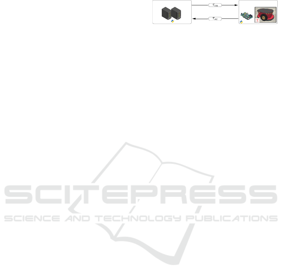
The basic architecture of the experimental setup is

shown in Figure 1. The evaluation of the system is

carried out through two computers. The ﬁrst rep-

resents the edge computing side and performs as a

server. The second, located at the local side and at-

tached to the robot, act as the client, sending state

measurements and waiting for responses from the

server containing the control sequence input. For both

sides, the communication protocol used to deliver and

receive packets is the UDP.

The robot used is the Pioneer 3-DX and is sim-

ulated in the CoppeliaSim (Rohmer et al., 2013).

Through an Application Programming Interface

Edge Side Local Side

Figure 1: Basic architecture of the experimental setup.

(API), the CoppeliaSim is linked to the local side

through a TCP/IP socket. Note that the CoppeliaSim

runs in a computer over an operating system; how-

ever, since the tool is simulating the robot at the local

side, the computer associated is considered to have

limited computing capabilities, but can run the sen-

sor and actuator routines, and can send/receive data

by the communication network. Suppose that a phys-

ical robot would be used. In this case, the computer

which simulates the robot in CoppeliaSim would be

changed by a physical robot attached to a computer

with limited resources (e.g., a Raspberry Pi) or even a

microcontroller.

The ﬂowcharts of Figure 2(a) and 2(b), respec-

tively, describes how the edge code and the sen-

sor thread of the local code works. Both software

executed at the edge and local sides are written in

Python and are referred to as the edge code and lo-

cal code. The network delays are estimated through

timestamps. τ

in the edge code, while τ

is es-

timated by the local code and is given back to the

edge code. The edge and local clocks are assumed to

be synchronized. τ

mpc

is estimated during the MPC

optimization running. With these delays, the pre-

dictor can ﬁnally predicts the robot’s state and trig-

ger the MPC optimization problem solved through

CasADi (Andersson et al., 2019). The sensor sam-

pling interval is T (equal to the time step of the MPC

predictions).

The experimental procedure is facilitated by im-

plementing the edge and local side on the same com-

puter. However, the local code and CoppeliaSim

runs in the native operating system, while the edge

code runs in a Linux virtual machine. The virtu-

alization software creates the virtual network inter-

face between the native and virtualized operating sys-

tem. The ERRANT (EmulatoR of Radio Access NeT-

works) developed by Trevisan et al. (2020) and the

Linux NetEm (Network Emulator) has been adopted

to emulate some network proﬁles. The ERRANT is

an open-source tool that emulates mobile networks

based on a data set composed of real measurements

and runs on top of NetEm. That tool was used in

this work to emulate the 3G and 4G networks. The

NetEm was also purely applied to emulate a network

with packet loss and a 5G network. The network em-

ulation was carried out in the virtual machine at the

local side. More details about the overall system op-

eration are discussed in Section 4.

CLOSER 2021 - 11th International Conference on Cloud Computing and Services Science

298

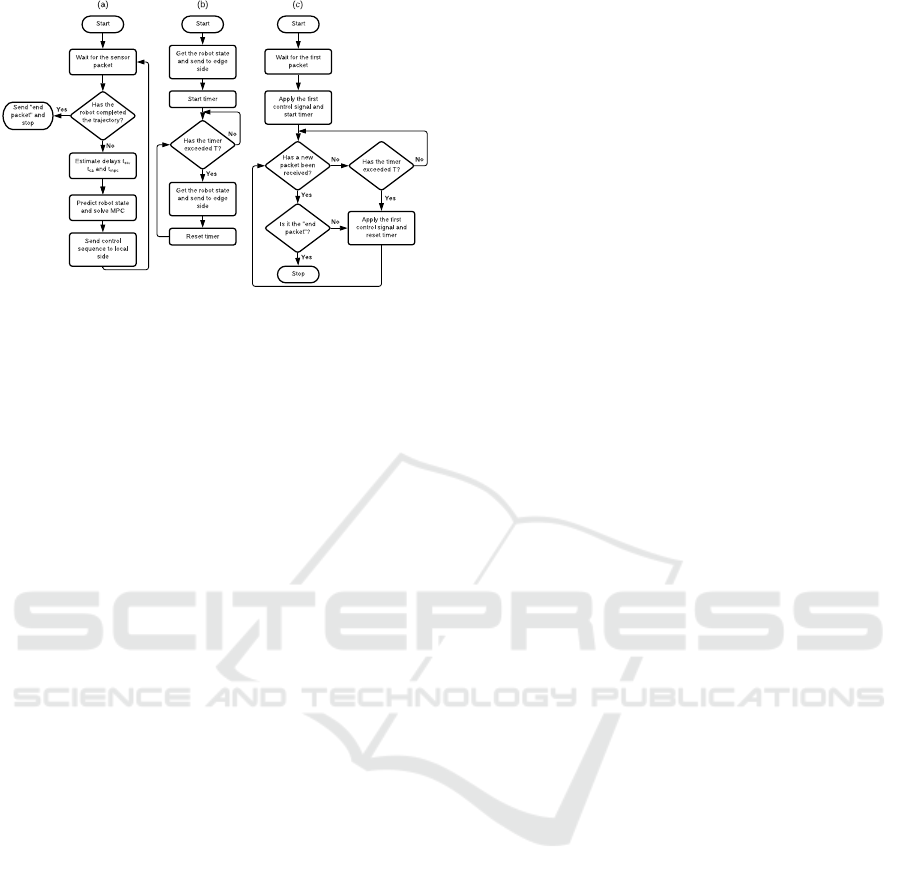
Figure 2: Flowchart describing the operation of: (a) Edge

code, (b) and (c) the sensor thread and the compensation

strategy of the local code, respectively.

3.1 Model Predictive Control

The MPC, sometimes referred to as Receding Hori-

zon Control, obtains control actions by solving a ﬁnite

horizon open-loop optimal control problem at each

sampled state. The plant’s measured state is taken as

the initial state for the optimization problem, calcu-

lated within a prediction horizon N. This MPC pro-

cedure makes it different from conventional control,

on what a pre-computed control law is adopted. The

MPC can deal with constraints, deﬁning limits for the

plant state’s control input and safety limits. Another

essential feature is the capability to control a multi-

variable process (Mayne et al., 2000).

The optimization problem is determined to mini-

mize the following cost function J:

minimize

J =

N−1

∑

k=0

(k)Qx(k) + u

(k)Ru(k) (1)

subject to g1 ≤ G1 and g2 = G2

where x(k) and u(k) denotes the state and the control

input, respectively. The diagonal matrix Q penalizes

the difference between the predicted state and the ref-

erence, while the matrix R does the same with the con-

trol input. G

and G

are, respectively, the inequality

and equality constraints. The basic MPC (Bemporad

and Morari, 1999) so runs repeatedly the following

sequence:1) get the new state x(k); 2) solve the opti-

mization problem (1); 3) apply only u(k) = u(k +0|k);

4) make k ← k + 1 and go to step 1.

3.2 Compensation Strategy

The compensation strategy for the network delay and

packet loss is deployed in the local code and is brieﬂy

represented by the ﬂowchart of Figure 2(c). After the

local code has started, it waits for the ﬁrst packet com-

ing from the edge side. When received, it applies the

ﬁrst control signal of the sequence generated by the

MPC and start the timer. Whenever a new packet has

arrived, the ﬁrst control signal is applied and the timer

is reset. If the packet is delayed or lost and the time

exceeds T, the next control signal is applied and the

timer is again reset. If the last control signal has been

reached, it continues being applied until a new packet

is received. The “end packet” is a packet sent by the

edge side when the robot has completed the trajectory.

It is sent several times to ensure that it will reach the

other side in case of packet losses.

3.3 Mobile Robot

The differential driving mobile robot, classiﬁed as

a non-holonomic mobile robot, may have two rear

wheels and a front castor wheel, or a four-wheel

conﬁguration. The two wheels conﬁguration is used

here. Details of the kinematic equation can be seen

in Dongbing Gu and Huosheng Hu (2006).

The state and control signal vectors are respec-

tively denoted as x = [x y θ]

and u = [v ω]

. The

state variables x and y represents the Cartesian posi-

tion in meters of the robot, and θ is the robot orienta-

tion in radians referenced from the x axis. The control

variables are the linear speed v, in meters per second,

and the angular speed ω, in radians per second. The

robot’s linear and angular speeds depends on the left

and right wheel speeds and the distance between the

wheels.

4 VALIDATION

The validation procedure was based on tests con-

ducted by Dongbing Gu and Huosheng Hu (2006)

and Mehrez et al. (2013), whose MPC is applied to

control a wheeled mobile robot. The same control

objectives are adopted here, which are Point Stabi-

lization and Trajectory Tracking. The items included

in the CoppeliaSim scene are the Pioneer 3-DX robot

and a ﬂoor with dimensions 25x25 m, where x and y

covers the intervals from -12.5 to 12.5 m.

It’s important to note that, for now, the main idea

is to validate the compensation strategy detailed in

the previous section. The trajectories followed by the

AGV during the validation are not necessarily a real

case of the Industry 4.0 or any other application, but is

enough to evaluate the controlling of the AGV at dis-

tinct network conditions, including favorable condi-

tions, the case of a 5G network, or bad conditions, the

case of a network with high delays and packet losses.

An Approach to Reduce Network Effects in an Industrial Control and Edge Computing Scenario

299

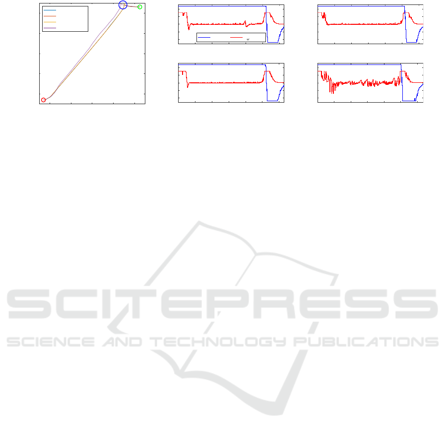
4.1 Point Stabilization

For the Point Stabilization simulations, the robot

should leave from the initial state x

and stabilize at

the desired reference x

. The vectors were adjusted as

= [−11.5 − 11.5 0]

and x

= [11.5 11.5 π]

for

all the simulations. If the reference orientation an-

gle is chosen π, the robot should maneuver near to

the state constraints and, thus, the MPC performance

in this circumstance can be evaluated. The controller

time step was set as T = 40 ms and the prediction

horizon size as N = 40, resulting in a prediction hori-

zon of 1600 ms in time. The sensor sampling period is

made equal to T. The state constraints imposed to the

MPC are −12.5 ≤ x ≤ 12.5 m and −12.5 ≤ y ≤ 12.5

m, which coincides with the ﬂoor dimensions set in

the CoppeliaSim scene. For the control signals, the

constraints are −1.2 ≤ v ≤ 1.2 m/s and −π/4 ≤ ω ≤

π/4 rad/s for the linear and angular speeds, respec-

tively.

Four network proﬁles have been taken an account

to evaluate the robot controlling in different network

conditions. The 3G and 4G networks were emulated

through the ERRANT. Since the tool emulates the

network based on a data set of real measurements,

there are different bandwidth and latency situations

for a single network technology, which could be re-

lated to the signal quality, for example. In this case,

for the 3G and 4G proﬁles, the network conditions

were conﬁgured to change every 5 seconds. The

NeTem purely was used to emulate the two other pro-

ﬁles. For the 5G proﬁle, no changes have been applied

to bandwidth, and the whole bandwidth of the Giga-

bit virtualized network interface is available. The up-

link and downlink delay was adjusted to 0.5 ms with a

normal distribution of 0.05 ms, resulting in a total la-

tency of 1 ms. The other proﬁle, called 200msPL50%,

has 100 ms of delay per channel, with a normal dis-

tribution of 10 ms, totalizing a latency of 200 ms.

The same proﬁle has 50% of packet losses per chan-

nel. The weights of the MPC cost function are de-

ﬁned as diagonal matrixes and were adjusted to Q =

diag(20,20,30) and R = diag(20,60). The two ﬁrst el-

ements of Q penalizes the states x and y, while the

last does with θ. For R, the ﬁrst and second elements

penalize the linear and angular speeds control signals,

respectively.

In Figure 3(a) is shown the trajectory of the robot

obtained for all the network proﬁles. The red circle

circumscribes the region where is the initial point, and

the green circle, the ﬁnal point. The blue circle delim-

its the region where the robot maneuver to stabilizes

in the desired reference. The maneuver occurs be-

cause the reference angle is set as π, and, in this case,

the robot should turn left and apply a reverse speed to

reach the ﬁnal point.

The control signals related to the linear and an-

gular speeds, applied to the robot, for each network

proﬁle, are shown in Figure 3(b) to 3(e). The sim-

ulations were programmed to end when the absolute

value of the difference between the reference and the

state vectors’ norms was less or equal to 0.2. This

occurred after approximately 32 s.

About the compensation strategy implemented by

the actuator in the local side, the biggest step in the

control sequence (for a prediction horizon of N = 40)

was to the 4

element (starting from zero) for the 5G

proﬁle. It means that, at one or more particular mo-

ments of the simulation, the local side remained four

times the controller’s time step (T ) without receiving

a new packet. Thus, the actuator has continued ap-

plying the control signals of the sequence generated

by the MPC until the arrival of a new packet with a

more recently calculated control sequence. For the

4G and 3G proﬁles, the advancing has been to the

and 15

elements, respectively. As expected, the

control signal sequence steps would be bigger in the

200msPL50% proﬁle, once a percentage of the pack-

ets are lost. In this case, the actuator advanced until

the 25

element. Even with the delays and packet

losses, the MPC combined with the compensation

strategy can stabilize the robot at the desired refer-

ence.

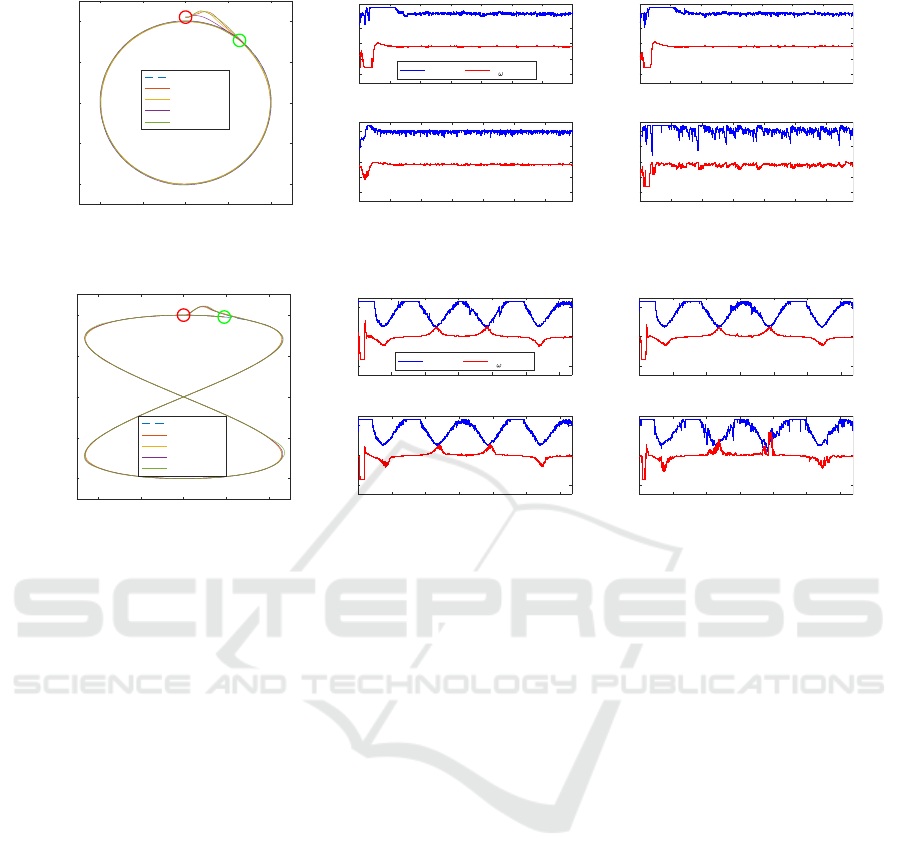
4.2 Trajectory Tracking

In the Trajectory Tracking, all the simulations pro-

cedures and adjustments were the same, except for

the reference. Now, the reference vector is not

ﬁxed, but is time varying. Two trajectories with

different shapes were simulated, the circular-shape

and eight-shape. The reference vector is given by

= [x(t) y(t) θ(t)]

. For the circular-shape, x(t) and

y(t) are calculated by x

(t) and y

(t) from (2). x

(t)

and y

(t) from the same equation are used for the

eight-shape. For both shapes, θ(t) is calculated by

(3), where T is the controller time step.

(t) = 10.0 sin(0.1t) x

(t) = 11.5 sin(0.1t)

(t) = 10.0 cos(0.1t) y

(t) = 10.0 cos(0.05t)

(2)

θ(t) = arctan

y(t+T )−y(t)

x(t+T )−x(t)

(3)

Another difference for the Trajectory Tracking is how

the MPC cost function is calculated. The cost func-

tion now takes an account not only a reference point

but rather a vector containing N points (remember

that N is the prediction horizon size). This approach

so brings better results once the controller can “see”

CLOSER 2021 - 11th International Conference on Cloud Computing and Services Science

300

-10 -5 0 5 10

x (m)

-10

-5

y (m)

(a) Trajectory in Point Stabilization

200msPL50%

0 5 10 15 20 25 30

time (s)

-1

-0.5

0.5

Control Signal

(b) 3G

(m/s) u (rad/s)

0 5 10 15 20 25 30

time (s)

-1

-0.5

0.5

Control Signal

0 5 10 15 20 25 30

time (s)

-1

-0.5

0.5

Control Signal

(d) 5G

0 5 10 15 20 25 30

time (s)

-1

-0.5

0.5

Control Signal

(e) 200msPL50%

Figure 3: Point stabilization results for all the network proﬁles: (a) Trajectory of the robot, (b)–(e) Control signals.

the future trajectory and suitably calculate the control

signal sequence. On the other hand, the processing

time increases. The prediction horizon was reduced to

N = 30, and the controller time step and sensor sam-

pling period were increased to T = 80 ms to reduce

the impact of that. One exception was considered for

the simulation’s prediction horizon size with the 5G

proﬁle, adjusted to N = 20, as the network conditions

are much more favorable. In this case, the controller’s

advancing into the future can be smaller, reducing the

MPC processing time.

For both trajectory shapes in all the network

proﬁles, the Q weights were adjusted to Q =

diag(30,30,0.2), except in the 200msPL50% proﬁle,

where it was adjusted to Q = diag(40,40,0.2). For

the circular-shape, the R weight was set as R =

diag(50,50) in all the simulations. In case of the

eight-shape, the R diagonal matrix received the val-

ues R = diag(10,5) for the three ﬁrst proﬁles and R =

diag(20,20) for the 200msPL50% proﬁle.

The trajectory of the robot for the circular-shape

and all network proﬁles, can be seen in Figure 4(a),

whereas the controls signals are depicted in Fig-

ure 4(b) to 4(e). The red circle delimits the re-

gion of the initial state, denoted by the vector

= [0 10.5 0]

. The initial state is outside the circu-

lar perimeter; however, the controller quickly moves

the robot to the reference trajectory, even more in the

5G proﬁle. The robot completes the trajectory in the

clockwise direction and starts a new lap, but immedi-

ately stops in the region delimited by the green cir-

cle. The simulation was programmed to end after

70 s, time enough to complete a lap, and complete

the beginning of a new one. The same procedures

were repeated with the eight-shape, and the results

can be seen in Figure 5. In this case, the initial state is

= [0 10 0]

and the simulation time was adjusted

to 130 s.

The circular-shape trajectory is smoother and eas-

ier to follow, as maintaining constant the linear and

angular speeds are enough to keep the robot in the

reference trajectory. Oppositely, in the eight-shape,

the controller should continuously make changes in

the linear and angular speeds. Nevertheless, even in

bad network conditions, the trajectory is successfully

followed and are very similar for all the network pro-

ﬁles. As expected, Trajectory Tracking has better re-

sults because the controller considers the future tra-

jectory to generate the control sequence. Therefore,

even if the packets forwarded to the local side are de-

layed or lost, the MPC’s predictive nature can gen-

erate a control sequence exploited by the actuator to

keep the robot in the desired reference.

If a path planner is adopted, the planned path can

be provided to the MPC and the Trajectory Tracking

method can be used. In the same way, the actuator in

the local side will be able to make the compensations

when necessary and track the robot in the planed path.

5 CONCLUSIONS

This paper introduced an experimental setup of a sys-

tem for compensation of delays and packet loss in

communication networks. In the proposed system,

Edge computing supports the MPC execution to con-

trol a mobile robot. The actuator uses the control se-

quence generated by the MPC, within the prediction

horizon to compensate. We implemented two control

objectives: Point Stabilization and Trajectory Track-

ing. In the ﬁrst, the robot should leave from an ini-

tial state and reach the reference. The second repre-

sents this work’s main contribution since the future

trajectory points are included in the MPC optimiza-

tion problem. The control sequence is, in this case,

generated according to the future trajectory. The ac-

tuator takes advantage of the last received control se-

quence when the packets from the edge are delayed

or lost. Thus the control signals are continuously ap-

plied to the robot. The favorable conditions of the 5G

network allow the reduction of the prediction horizon,

and consequently, the MPC has a faster response.

An Approach to Reduce Network Effects in an Industrial Control and Edge Computing Scenario

301

-10 -5 0 5 10

x (m)

-10

-5

y (m)

(a) Trajectory Tracking - Circular-shape

Reference

200msPL50%

0 10 20 30 40 50 60

time (s)

-1

-0.5

0.5

Control Signal

(b) 3G

(m/s) u (rad/s)

0 10 20 30 40 50 60

time (s)

-1

-0.5

0.5

Control Signal

0 10 20 30 40 50 60

time (s)

-1

-0.5

0.5

Control Signal

(d) 5G

0 10 20 30 40 50 60

time (s)

-1

-0.5

0.5

Control Signal

(e) 200msPL50%

Figure 4: Circular-shape results for all the network proﬁles: (a) Trajectory of the robot, (b)–(e) Control signals.

-10 -5 0 5 10

x (m)

-10

-5

y (m)

(a) Trajectory Tracking - Eight Shape

Reference

200msPL50%

0 20 40 60 80 100 120

time (s)

-1

Control Signal

(b) 3G

(m/s) u (rad/s)

0 20 40 60 80 100 120

time (s)

-1

Control Signal

0 20 40 60 80 100 120

time (s)

-1

Control Signal

(d) 5G

0 20 40 60 80 100 120

time (s)

-1

Control Signal

(e) 200msPL50%

Figure 5: Eight-shape results for all the network proﬁles: (a) Trajectory of the robot, (b)–(e) Control signals.

The next steps may comprise a more realistic scenario

of Industry 4.0, including multiple AGV’s using path

planning, including autonomous interactions between

AGV’s and other actors of the manufacturing pro-

cess. The use of Edge Computing may support those

mentioned tasks, but also other relevant ones, like,

change the parameters of the controller according to

the load characteristics (e.g., dimensions, weight, and

fragility), promote the cooperation among multiple

AGV’s to transport a heavier load, use Artiﬁcial Intel-

ligence to help on the decision-making and other tasks

that requires more computing power. Edge Comput-

ing also helps to reduce the cost with the robots and

all devices and machinery related to the industrial en-

vironment, given that the computing power will be

placed at the edge, besides, the battery consumption

of the mobile robots may be reduced.

ACKNOWLEDGEMENTS

The authors thank the support of the Coordenac¸

de Aperfeic¸oamento de Pessoal de N

ıvel Superior -

Brazil (CAPES), and Programa de P

os-Graduac¸

ao em

Engenharia El

etrica (COPELE), Federal University of

Campina Grande.

REFERENCES

Aazam, M., Zeadally, S., and Harras, K. A. (2018). De-

ploying fog computing in industrial internet of things

and industry 4.0. IEEE Transactions on Industrial In-

formatics, 14(10):4674–4682.

Abbas, N., Zhang, Y., Taherkordi, A., and Skeie, T. (2018).

Mobile edge computing: A survey. IEEE Internet of

Things Journal, 5(1):450–465.

Abdelzaher, T., Hao, Y., Jayarajah, K., Misra, A., Skarin, P.,

Yao, S., Weerakoon, D., and

Arz

en, K.-E. (2020). Five

challenges in cloud-enabled intelligence and control.

ACM Trans. Internet Technol., 20(1).

Al-Fuqaha, A., Guizani, M., Mohammadi, M., Aledhari,

M., and Ayyash, M. (2015). Internet of things: A

survey on enabling technologies, protocols, and ap-

plications. IEEE Communications Surveys Tutorials,

17(4):2347–2376.

Andersson, J. A. E., Gillis, J., Horn, G., Rawlings, J. B.,

and Diehl, M. (2019). CasADi: a software framework

for nonlinear optimization and optimal control. Math-

ematical Programming Computation, 11(1):1–36.

Bemporad, A. and Morari, M. (1999). Robust model predic-

tive control: A survey. In Garulli, A. and Tesi, A., ed-

itors, Robustness in identiﬁcation and control, pages

207–226, London. Springer London.

Chen, B., Wan, J., Celesti, A., Li, D., Abbas, H., and Zhang,

Q. (2018). Edge computing in iot-based manufac-

turing. IEEE Communications Magazine, 56(9):103–

109.

Chen, C., Lyu, L., Zhu, S., and Guan, X. (2020). On-

CLOSER 2021 - 11th International Conference on Cloud Computing and Services Science

302

demand transmission for edge-assisted remote control

in industrial network systems. IEEE Transactions on

Industrial Informatics, 16(7):4842–4854.

Dongbing Gu and Huosheng Hu (2006). Receding

horizon tracking control of wheeled mobile robots.

IEEE Transactions on Control Systems Technology,

14(4):743–749.

Esen, H., Adachi, M., Bernardini, D., Bemporad, A., Rost,

D., and Knodel, J. (2015). Control as a service

(caas): Cloud-based software architecture for automo-

tive control applications. In Proceedings of the Second

International Workshop on the Swarm at the Edge of

the Cloud, page 13–18, New York, NY, USA.

Findeisen, R. and Varutti, P. (2009). Stabilizing Nonlinear

Predictive Control over Nondeterministic Communi-

cation Networks, pages 167–179. Springer Berlin Hei-

delberg, Berlin, Heidelberg.

une, L., Allg

ower, F., Findeisen, R., Fischer, J., Groß, D.,

Hanebeck, U. D., Kern, B., M

uller, M. A., Pannek, J.,

Reble, M., Stursberg, O., Varutti, P., and Worthmann,

K. (2014). Distributed and Networked Model Predic-

tive Control, pages 111–167. Springer International

Publishing, Heidelberg.

Gubbi, J., Buyya, R., Marusic, S., and Palaniswami, M.

(2013). Internet of things (iot): A vision, architectural

elements, and future directions. Future Generation

Computer Systems, 29(7):1645 – 1660.

Hegazy, T. and Hefeeda, M. (2015). Industrial automation

as a cloud service. IEEE Transactions on Parallel and

Distributed Systems, 26(10):2750–2763.

Hespanha, J. P., Naghshtabrizi, P., and Xu, Y. (2007). A

survey of recent results in networked control systems.

Proceedings of the IEEE, 95(1):138–162.

Hojjat A. Izadi, B. W. G. and Zhang, Y. (2011). Decentral-

ized model predictive control for cooperative multiple

vehicles subject to communication loss. International

Journal of Aerospace Engineering, 2011:1–13.

Kaur, K., Garg, S., Aujla, G. S., Kumar, N., Rodrigues, J. J.

P. C., and Guizani, M. (2018). Edge computing in the

industrial internet of things environment: Software-

deﬁned-networks-based edge-cloud interplay. IEEE

Communications Magazine, 56(2):44–51.

Kiani, A. and Ansari, N. (2018). Edge computing aware

noma for 5g networks. IEEE Internet of Things Jour-

nal, 5(2):1299–1306.

Liu, G., Xia, Y., Chen, J., Rees, D., and Hu, W. (2007).

Networked predictive control of systems with random

network delays in both forward and feedback chan-

nels. IEEE Transactions on Industrial Electronics,

54(3):1282–1297.

Mayne, D., Rawlings, J., Rao, C., and Scokaert, P. (2000).

Constrained model predictive control: Stability and

optimality. Automatica, 36(6):789 – 814.

Mehrez, M. W., Mann, G. K. I., and Gosine, R. G. (2013).

Stabilizing nmpc of wheeled mobile robots using

open-source real-time software. In 2013 16th Inter-

national Conference on Advanced Robotics (ICAR),

pages 1–6.

Pallasch, C., Wein, S., Hoffmann, N., Obdenbusch, M.,

Buchner, T., Waltl, J., and Brecher, C. (2018). Edge

powered industrial control: Concept for combining

cloud and automation technologies. In 2018 IEEE In-

ternational Conference on Edge Computing (EDGE),

pages 130–134.

Pin, G. and Parisini, T. (2011). Networked predictive con-

trol of uncertain constrained nonlinear systems: Re-

cursive feasibility and input-to-state stability analysis.

IEEE Transactions on Automatic Control, 56(1):72–

87.

Qiu, T., Chi, J., Zhou, X., Ning, Z., Atiquzzaman, M.,

and Wu, D. O. (2020). Edge computing in indus-

trial internet of things: Architecture, advances and

challenges. IEEE Communications Surveys Tutorials,

22(4):2462–2488.

Rimal, B. P., Van, D. P., and Maier, M. (2017). Mobile

edge computing empowered ﬁber-wireless access net-

works in the 5g era. IEEE Communications Magazine,

55(2):192–200.

Rohmer, E., Singh, S. P. N., and Freese, M. (2013). V-rep:

A versatile and scalable robot simulation framework.

In 2013 IEEE/RSJ International Conference on Intel-

ligent Robots and Systems, pages 1321–1326.

Sisinni, E., Saifullah, A., Han, S., Jennehag, U., and Gid-

lund, M. (2018). Industrial internet of things: Chal-

lenges, opportunities, and directions. IEEE Transac-

tions on Industrial Informatics, 14(11):4724–4734.

Skarin, P., Eker, J., Kihl, M., and

Arz

en, K.-E. (2019).

Cloud-assisted model predictive control. In 2019

IEEE International Conference on Edge Computing

(EDGE), pages 110–112.

Skarin, P., T

arneberg, W.,

Arzen, K., and Kihl, M. (2018).

Towards mission-critical control at the edge and over

5g. In 2018 IEEE International Conference on Edge

Computing (EDGE), pages 50–57.

Trevisan, M., Safari Khatouni, A., and Giordano, D. (2020).

ERRANT: Realistic emulation of radio access net-

works. Computer Networks, 176:107289.

Ulusoy, A., Gurbuz, O., and Onat, A. (2011). Wire-

less model-based predictive networked control system

over cooperative wireless network. IEEE Transactions

on Industrial Informatics, 7(1):41–51.

Vick, A., Guhl, J., and Kr

uger, J. (2016). Model predic-

tive control as a service — concept and architecture

for use in cloud-based robot control. In 2016 21st

International Conference on Methods and Models in

Automation and Robotics (MMAR), pages 607–612.

Wan, J., Tang, S., Shu, Z., Li, D., Wang, S., Imran, M., and

Vasilakos, A. V. (2016). Software-deﬁned industrial

internet of things in the context of industry 4.0. IEEE

Sensors Journal, 16(20):7373–7380.

Xu, H., Yu, W., Grifﬁth, D., and Golmie, N. (2018). A sur-

vey on industrial internet of things: A cyber-physical

systems perspective. IEEE Access, 6:78238–78259.

Yaqoob, I., Ahmed, E., Hashem, I. A. T., Ahmed, A. I. A.,

Gani, A., Imran, M., and Guizani, M. (2017). Internet

of things architecture: Recent advances, taxonomy,

requirements, and open challenges. IEEE Wireless

Communications, 24(3):10–16.

Zhao, P. and D

an, G. (2018). A benders decomposi-

tion approach for resilient placement of virtual pro-

cess control functions in mobile edge clouds. IEEE

Transactions on Network and Service Management,

15(4):1460–1472.

An Approach to Reduce Network Effects in an Industrial Control and Edge Computing Scenario

303