
Performance Analysis of Different Operators in Genetic Algorithm for
Solving Continuous and Discrete Optimization Problems
Shilun Song
1
, Hu Jin
1
and Qiang Yang
2,∗
1
Department of Electrical and Electronic Engineering, Hanyang University, Ansan, 15588, South Korea
2
School of Artificial Intelligence, Nanjing University of Information Science and Technology, Nanjing 210044, China
Keywords:
Genetic Algorithm, Nonlinear Optimization, Traveling Salesman Problem.
Abstract:
Genetic algorithm (GA), as a powerful meta-heuristics algorithm, has broad applicability to different opti-
mization problems. Although there are many researches about GA, few works have been done to synthetically
summarize the impact of different genetic operators and different parameter settings on GA. To fill this gap,
this paper has conducted extensive experiments on GA to investigate the influence of different operators and
parameter settings in solving both continuous and discrete optimizations. Experiments on 16 nonlinear opti-
mization (NLO) problems and 9 traveling salesman problems (TSP) show that tournament selection, uniform
crossover, and a novel combination-based mutation are the best choice for continuous problems, while roulette
wheel selection, distance preserving crossover, and swapping mutation are the best choices for discrete prob-
lems. It is expected that this work provides valuable suggestions for users and new learners.
1 INTRODUCTION
Since Holland (Holland, 1992) came up with the first
generation of GA in 1975, GA and its variants have
been used in many fields, like traveling salesman
problems(Wang et al., 2020), wireless sensor net-
work(Zorlu et al., 2017), feature selection(Li et al.,
2009)(Huang et al., 2010), etc. However, few re-
search exists on discussing in detail the impact of dif-
ferent operators and parameters on the performance
of GA.
As shown in figure 1, there are mainly three types
of operators in GA: selection operator, crossover op-
erator, and mutation operator. The selection operator
mainly chooses promising parents for the crossover
operator. The crossover operator aims to exchange the
information of parent individuals to generate new off-
spring. The mutation operator is to generate new val-
ues of variables based on some rules. By repeatedly
applying these three operators, the optima of prob-
lems may be found.
To comprehensively investigate the performance
of different operators and parameters in GA, we con-
duct extensive experiments on both continuous and
discrete problems. Specifically, on continuous prob-
lems, we use the nonlinear optimization (NLO) prob-
∗
Corresponding author.
Start
Initialization
Evaluation Selection
CrossoverMutation
End Condition
End
Yes
No
Figure 1: The overall framework of genetic algorithm (GA).
lems as the representatives to conduct experiments,
while on discrete problems we use the traveling sales-
man problems (TSP) as the representatives.
In the literature, there are some researches work-
ing on the comparison of selection operators (Zhong
et al., 2005) (Chen et al., 2020), crossover operators
(Pinho and Saraiva, 2020), and the combinations of
crossover and mutation operators (Hildayanti et al.,
2018) on NLO. For TSP problems, researchers have
also developed many variants of GA from different
perspectives, like improvement for selection opera-
tors (Yu et al., 2016), crossover operators (Freisleben
536
Song, S., Jin, H. and Yang, Q.
Performance Analysis of Different Operators in Genetic Algorithm for Solving Continuous and Discrete Optimization Problems.
DOI: 10.5220/0010494005360547
In Proceedings of the 23rd International Conference on Enter prise Information Systems (ICEIS 2021) - Volume 1, pages 536-547
ISBN: 978-989-758-509-8
Copyright
c
2021 by SCITEPRESS – Science and Technology Publications, Lda. All rights reserved

and Merz, 1996), mutation operators (Zhou and Song,
2016), and the combination of the above two opera-
tors (Yu et al., 2011).
Different from existing studies, this paper aims to
give a full-scale introduction and analysis of different
operators and parameter settings on GA.
The remainder of this paper is organized as fol-
lows. In section 2, we discuss the continuous and
discrete optimization problems. Then, in section 3,
we show the involved genetic operators for the two
types of problems in detail. In section 4, numerical
experiments are conducted to show the performance
of different operators. Finally, we give the conclusion
in section 5.
2 CONTINUOUS AND DISCRETE
OPTIMIZATION PROBLEMS
2.1 Continuous Optimization Problem
In the real world, NLO widely exists in many fields
in different forms, like autonomous surface vehicles
(Eriksen and Breivik, 2017), optimal placement prob-
lems (Almunif and Fan, 2017), and signal source lo-
calization (Ma et al., 2017), etc. This kind of prob-
lems become considerably difficult to solve as the di-
mensionality increases (Yang et al., 2020). Except for
GA, there are also researches which apply other evo-
lutionary algorithms to solve this type of problems,
just like ant colony optimization (Yang et al., 2017b)
and estimation of distribution algorithms (Yang et al.,
2017a).
The target of NLO is expected to achieve the opti-
mal solution under some restrictions, and the feasible
solutions are taken from the continuous set. NLO can
be noted as
maximize/minimize f (x),
sub ject to x ∈ X
where f (x) is a nonlinear objective function, and X
is the domain of the target function . For the conve-
nience of discussion, we note the feasible solution x
as an M-dimensional vector (x
1
,x
2
,. ..,x
M
).
Based on the property that whether there are mul-
tiple optima in the solution space, NLO is roughly
categorized into two types: unimodal problems and
multimodal problems.
• Unimodal Problem. There is only one optimum,
namely the global optimum, for this kind of prob-
lems, as shown in figure 2. Such a property leads
to that this type of problems is relatively easy to
solve.
Figure 2: An example of unimodal functions.
• Multimodal Problem. As shown in figure 3,
there are more than one local optima around the
global one. This type of problems is more com-
mon and complex in the real world applications.
Thus, we pay more attention to this type of func-
tions.
Figure 3: An example of multimodal functions.
2.2 Discrete Optimization Problem
TSP is a typical and complex kind of discrete prob-
lems. Many optimization problems in real-world ap-
plications could be modeled as TSP, like multi-bridge
machining schedule (Li et al., 2017), 3-D printing
(Ganganath et al., 2016) and unmanned aircraft sys-
tems (Xie et al., 2019).
Let V = {v
1
,v
2
,. ..,v
M
} be the city set, where v
i
represents the city indexed by i. The cost from city
i to j is noted as c
i j
. For simplicity, the problems
in the following discussion are limited to symmetric
TSP, which means that c
i j
= c
ji
for ∀i, j.
Likewise, we note a route as x = (x
1
,x
2
,. ..,x
M
),
whose total distance is noted as
f (x) =
M
∑
i=1
c
x
i
x
i+1
where x
M+1
= x
1
. The purpose is to search for the
optimal route which brings the minimal cost. Figure
4 shows the optimal route for the a280 instance. Our
example data comes from TSPLIB (http://elib.zib.de/
pub/mp-testdata/tsp/tsplib/tsp/index.html).
Performance Analysis of Different Operators in Genetic Algorithm for Solving Continuous and Discrete Optimization Problems
537

0 50 100 150 200 250 300
x
0
50
100
150
y
a280.tsp
Figure 4: The optimal route of a280.
3 GENETIC OPERATORS
In this part, related evolutionary operators are dis-
cussed. Suppose there are N individuals that get in-
volved in the evolution. The whole population is
noted as U = {u
1
,u
2
,. ..,u
N
}. The fitness value of in-
dividual u
i
is noted as α
i
. All fitness values are listed
in the fitness value vector Θ = (α
1
,α
2
,. ..,α
N
).
3.1 Encoding Method
3.1.1 NLO Encoding
For NLO, each dimension of the chromosome is
coded with a real number within the feasible range.
As a consequence, each chromosome represents a fea-
sible solution in the solution space.
3.1.2 TSP Encoding
The chromosome for TSP is set as a permutation of
the cities. For example, a feasible solution of 9-city
TSP is shown in figure 5.
9 4 7 5 3 6 1 8 2
Figure 5: A chromosome of GA when solving a TSP in-
stance with 9 cities.
3.2 Initialization Operator
3.2.1 NLO Initialization
As for NLO, the genes are randomly sampled in the
corresponding value ranges.
3.2.2 TSP Initialization
For TSP, the greedy method is used to initialize the
routes as shown in algorithm 1.
Algorithm 1: TSP Initialization.
Input: the number of cities M.
Output: a new route r
1
r
2
.. .r
M
.
1: Initialization: an empty route
2: Randomly choose a city v
0
1
3: r
1
← v
0
1
4: for i = 2 to M do
5: Choose the city v
0
i
that is the nearest to v
0
i−1
and not included in the route yet.
6: r
i
← v
0
i
7: end for
3.3 Selection Operator
Considering that the selection operators can be com-
monly used in both continuous and discrete problems,
there is no need to discuss them respectively. In this
paper, the following two selection operators are con-
cerned.
3.3.1 Roulette Wheel Selection (RWS)
This operator comes from the roulette game. In this
selection, the individuals with larger fitness values
have higher probabilities to be selected. The detailed
process of the roulette wheel selection is shown in al-
gorithm 2.
Algorithm 2: Roulette Wheel Selection (RWS).
Input: population U = {u
1
,u
2
,. ..,u
N
}, fitness
value vector Θ = {α
1
,α
2
,. ..,α
N
}.
Output: selected parents U
0
.
1: for i = 2 to N do
2: α
i
← α
i
+ α
i−1
3: end for
4: for i = 1 to N do
5: α
i
← α
i
/α
N
6: end for
7: α
0
← 0
8: r ← rand(0, 1). // Uniform[0, 1]
9: Find k s.t. r ∈ (α
k−1
,α
k
]
10: Record individual u
k
as a selected parent.
11: Go back to 8 until N parents are selected.
3.3.2 Tournament Selection (TS)
The main process of the tournament selection is
shown in algorithm 3. Obviously, a larger n
player
brings higher selection pressure to the population,
where individuals with poorer performance have
smaller probability to survive.
ICEIS 2021 - 23rd International Conference on Enterprise Information Systems
538

Algorithm 3: Tournament Selection (TS).
Input: population U = {u
1
,u
2
,. ..,u
N
}, fitness
value vector Θ = {α
1
,α
2
,. ..,α
N
}.
Output: selected parents U
0
.
1: for i = 1 to N do
2: Randomly select n
player
individuals.
3: Record the best individual as a selected
parent.
4: end for
3.4 Crossover Operator
The crossover operators are used for parents to gen-
erate their children from the microcosmic perspec-
tive. The combination of genes from parents brings
children different performance. We note p
x
as the
probability that an individual is selected. For every
couple of selected parent individuals, a correspond-
ing crossover operator is applied.
3.4.1 NLO Crossover
The crossover operators for NLO generate child indi-
viduals by letting the two chosen parents swap some
corresponding genes.
Single Point Crossover (SPoC). For SPoC, a po-
sition of the chromosome except for the first one is
randomly chosen, and all of the genes from that posi-
tion to the end are swapped. The process in detail is
shown in algorithm 4.
Algorithm 4: Single Point Crossover (SPoC).
Input: two parent chromosomes x
[1]
and x
[2]
.
Output: two child chromosomes.
1: Randomly choose a position k ∈ {2, .. .,M}
2: for i = k to M do
3: Swap x
[1]
i
and x
[2]
i
4: end for
Uniform Crossover (UC). For UC, the algorithm
checks every position and swaps the corresponding
genes with probability p
swap
. The process in detail is
shown in algorithm 5.
3.4.2 TSP Crossover
In TSP, the chromosome is a complete route, which
means the operators should not break the routing rule
of TSP. Two common operators called distance pre-
serving crossover (Freisleben and Merz, 1996) and
single piece crossover (Kaur and Murugappan, 2008)
are discussed as follow.
Algorithm 5: Uniform Crossover (UC).
Input: two parent chromosomes x
[1]
and x
[2]
.
Output: two child chromosomes.
1: for i = 1 to M do
2: if rand() < p
swap
then
3: Swap x
[1]
i
and x
[2]
i
4: end if
5: end for
Distance Preserving Crossover (DPC). DPC gen-
erates a set O where every element o
i
satisfies the fol-
lowing two conditions:
• o
i
is a sub-route of both parent routes.
• o
i
is not a sub-route of any common route piece in
both parent routes.
Then it completes the child routes via the greedy strat-
egy. The process of DPX is shown in figure 6
Parent 1
7 9 5 3 4 6 1 8 2
9 2 6 1 8 7 5 3 4
Parent 2
9 2 6 1 8 7 5 3 4
Set O
5 3 4 9 6 1 8 7 2
6 1 8 2 7 5 3 4 9
Child 1
Child 2
Figure 6: Distance preserving crossover.
Single Piece Crossover (SPiC). SPiC firstly selects a
corresponding continuous piece of the chromosomes
of the chosen parents, and then swaps the correspond-
ing piece, just as shown in figure 7.
Parent 1
9 4 7 5 3 6 1 8 2
9 2 6 1 8 7 5 3 4
Parent 2
6 1 8 7
Swapping
9 4 1 8 2
9 2 5 3 4
Child 1
Child 2
6 1 8 7
7 5 3 6
7 5 3 6
Figure 7: Single piece crossover.
3.5 Mutation Operator
3.5.1 NLO Mutation
In the mutation process, the algorithm checks all
genes in all chromosomes and applies the mutation
operator with probability p
m
.
Uniform Mutation (UM). The chosen gene ran-
domly switches to another value within the corre-
Performance Analysis of Different Operators in Genetic Algorithm for Solving Continuous and Discrete Optimization Problems
539

sponding value range. This method is helpful for the
algorithm to jump out of the local optimal areas, but
might kill the good feasible solution.
Exponential Mutation (EM). It brings a mutation
according to the fitness value of the individual. The
main idea is that the individual with a higher fitness
value should get a smaller mutation to keep the good
property and the poor individuals should get a bigger
mutation.
Let D
i
be the value range of the chosen gene x
i
,
and ~ is a random value generator that generates 1
with probability 0.5 and generates -1 with probability
0.5. Besides we note f(λ) as a random value gener-
ator whose value follows the exponential distribution
with parameter λ. Obviously, with a higher λ, the f
λ
is closer to 0 expectedly.
Algorithm 6 shows the process of the exponential
mutation operator for gene x
i
, where factor a and b
are parameters to control the mutation level.
Algorithm 6: Exponential Mutation (EM).
Input: gene x
i
, fitness value vector Θ.
Output: mutated gene x
0
i
.
1:
ˆ
α ← max(Θ)
2: λ ← b(α
i
/
ˆ
α)
a
3: δ ← ~f(λ) s.t. x
i
+ δ ∈ D
i
4: x
0
i
← x
i
+ δ ∈ D
i
Combination Mutation (CM). Basically, the expo-
nential mutation is a greedy strategy biased to good
individuals. However, the eliminated individuals with
poor performance may be also useful for the compu-
tation. Thus, we design a combination mutation op-
erator that applies the uniform mutation and the ex-
ponential mutation with the same probability. This is
supposed to decrease the influence of the greedy strat-
egy.
3.5.2 TSP Mutation
The mutation for TSP should not break the com-
pleteness of a route, and operators bringing overturn
are not supposed to be applied. In this paper, the
swap mutation (SM) and the simple inversion muta-
tion (SIM) are discussed.
Swap Mutation (SM). In this method, a probability
p
m
is used to select the mutation gene. The operator
swaps the cities on the chosen genes and their corre-
sponding nearest cities.
Simple Inversion Mutation (SIM). For every in-
dividual, once two positions on one of the route to
be mutated are chosen, the operator inverts the route
piece between the two positions, as shown in figure 8.
Before
Mutation
9 4 8 27 5 3 6 1
9 4 8 21 6 3 5 7
After
Mutation
Figure 8: Simple inversion mutation.
3.6 Accelerator: Elitist Strategy
This operator is set to get involved in every calcu-
lation as default. As is known, due to the random-
ness, the solution structure of every individual can
be changed with non-negligible probability, which
means that even the optimal individual may not be
kept and the searching speed of the algorithm gets
slow.
The elitist selection acts as follows: in every gen-
eration, the best individual is selected and gets com-
parison with the best one in the last generation. If
the current best individual performs better, it takes
place of the best one in the last generation. If not,
the best individual in the last generation takes place of
the worst individual in this generation. Thus, the best
individual until the current generation can always be
kept in the population.
Actually, it is checked that the number of kept
elites has no significant influence on the performance,
which means keeping the best one in every generation
is enough.
3.7 Local Search for TSP
As for TSP, local search is a necessary operator to
improve the solution accuracy. In this paper, we just
use 2-opt as the local search operator. It is also an
accelerator for the computation of TSP. The 2-opt op-
erator for an individual chromosome x
k
is shown in
algorithm 7.
3.8 The Complete GAs
Finally, we give the detailed process of the two com-
plete GAs: NLO-GA and TSP-GA.
Algorithm 8 shows the detailed process of GA for
NLO, and algorithm 9 shows the detailed process of
GA for TSP. GEN
MAX
, as the end controller, is the
number of generations for evolution. Step 3 of both
algorithms is used to record the individual with the
highest fitness value. It is the preparation for the eli-
tist selection. The overall difference between the two
ICEIS 2021 - 23rd International Conference on Enterprise Information Systems
540

Algorithm 7: 2-opt.
Input: chromosome x
k
, repeating time K.
Output: improved chromosome x
k
.
1: Compute the total distance f (x
k
)
2: x
0
k
← x
k
3: for i = 1 to N do
4: Randomly select two cities v
i
and v
j
5: Swap v
i
and v
j
on x
0
k
6: if f (x
0
k
) < f (x
k
) then
7: x
k
← x
0
k
8: end if
9: end for
GAs is the local search for TSP. In the next section,
we use these two schemes to test the performance of
genetic operators.
Algorithm 8: NLO-GA.
Input: population size N, maximum generation
GEN
MAX
, n
player
(if necessary), p
x
, p
swap
(if
necessary), p
m
.
Output: best individual u
opt
.
1: Initialize the population
2: Evaluate
3: Keep the best
4: for generation = 1 to GEN
MAX
do
5: Select
6: Crossover
7: Mutate
8: Evaluate
9: Keep the best and do the elitist strategy
10: end for
4 NUMERICAL EXPERIMENTS
In this section, we conduct numerical experiments to
compare genetic operators. Actually, it is hard to do
the theoretical analysis on which is the best opera-
tor. Our purpose is to find the suitable operators that
can obtain the best result under identical computation
costs.
Firstly, we introduce the details about all of the
experiments in subsection 4.1. With the numeri-
cal results, the comparisons of selection strategies,
crossover strategies, and mutation strategies are given
in subsection 4.2, 4.3, and 4.4, respectively.
4.1 Experiment Details
All algorithms are implemented in C language and
run on PC with Windows 10, CPU Intel Core i7-
8086K and RAM 64 GB.
Algorithm 9: TSP-GA.
Input: population size N, maximum generation
GEN
MAX
, n
player
(if necessary), p
x
, p
m
(if
necessary).
Output: best individual u
opt
.
1: Initialize the population
2: Evaluate
3: Keep the best
4: for generation = 1 to GEN
MAX
do
5: Select
6: Crossover
7: Mutate
8: Evaluate
9: Keep the best and do the elitist strategy
10: Local search
11: end for
4.1.1 Settings for NLO
For NLO, we select 4 functions shown in table 1
whose dimension can be easily expanded to high di-
mension.
Besides, for NLO-GA, parameter settings are
listed in table 2. Due to the randomness of the al-
gorithm, we use the average results over hundreds of
independent runs. The sample number in the table
means the repeating time.
4.1.2 Settings for TSP
For TSP, we select 9 instances of different sizes from
TSPLIB, which are listed in table 3. Besides, for TSP-
GA, some important and fixed parameter settings are
listed in table 4.
4.2 Selection Strategies Comparision
4.2.1 Selection Strategies in NLO
In this part, we mainly compare the performance of
RWS and TS on NLO. In the comparison, the SPoC
and UM are used as default crossover and mutation
operators. Under this setting, figures 18, 19, and 20
shows the performance of NLO-GA on 5, 15, and 30
dimensional problems.
4.2.2 Selection Strategies in TSP
In this part, we mainly compare the performance of
RWS and TS on TSP. In comparison, the DPC and
SM are used as default crossover and mutation oper-
ators. Under this setting, figures 9, 10, and 11 shows
the performance of TSP-GA on 50, 100, and 200 size
groups.
Performance Analysis of Different Operators in Genetic Algorithm for Solving Continuous and Discrete Optimization Problems
541

Table 1: NLO Instances.
Function Type Range Optima
f
1
= 1 +
∑
D
i=1
x
2
i
Unimodal [−100,100]
D
1
f
2
= 1 + 20 + e −20 exp
−0.2
q
∑
D
i=1
x
2
i
D
− exp
n
∑
D
i=1
cos(sπx
i
)
D
o
Multimodal [−32,32]
D
1
f
3
= 1 + D −
∑
D
i=1
cos(2πx
i
) −0.01 ∗ x
2
i
Multimodal [−5.12,5.12]
D
1
f
4
= 1 +
∑
D
i=1
y
2
i
− 10cos(2πy
i
) +10
,
where y
i
= x
i
if |x
i
| < 0.5 and y
i
=
round(2x
i
)
2
if |x
i
| ≥ 0.5.
Multimodal [−5.12,5.12]
D
1
Table 2: Parameter settings of NLO-GA.
Patameter Value
Population size 40
Tournament player 10
p
swap
for UC 0.5
Sample number 150
Table 3: TSP Instances.
Size Group Instance The Number of Cities
50
att48 48
eil51 51
berlin52 52
100
kroC100 100
eil101 101
lin105 105
200
rat195 195
d198 198
kroA200 200
4.2.3 Conclusion of Selection Strategies
According to the numerical results, we get the follow-
ing conclusions for solving NLO and TSP:
• For NLO, TS performs better than RWS. The
mutation probability p
m
makes significiant influ-
ence. With high dimension, TS needs a low p
m
to
achieve the best performance.
• For TSP, RWS is better, and it needs a small
crossover probability p
x
to find a relatively short
route.
4.3 Crossover Strategies Comparision
4.3.1 Crossover Strategies in NLO
In this part, we mainly compare the performance of
SPoC and UC on NLO. Actually, it is checked that
p
swap
does not make obvious influence on the compu-
tation. In the comparison, the TS and UM are used as
default selection and mutation operators. Under this
Table 4: Parameter settings of TSP-GA.
Patameter Value
Population size 60
Tournament player 15
p
m
for SM 0.1
2-opt time 10
Sample number (group 50&100) 300
Sample number (group 200) 100
setting, figures 21, 22, and 23 shows the performance
of NLO-GA on 5, 15, and 30 dimensional problems.
4.3.2 Crossover Strategies in TSP
In this part, we mainly compare the performance of
DPC and SPiC on TSP. In comparison, the RWS and
SM are used as default selection and mutation opera-
tors. Under this setting, figures 12, 13, and 14 shows
the performance of TSP-GA on 50, 100, and 200 size
groups.
4.3.3 Conclusion of Crossover Strategies
According to the numerical results, we get the follow-
ing conclusions for solving NLO and TSP:
• For NLO, the difference with respect to the per-
formance between the two crossover strategies is
not obvious.
• For TSP, DPC works better, and it also needs a
small crossover probability p
x
to find a relatively
short route.
4.4 Mutation Strategies Comparision
4.4.1 Mutation Strategies in NLO
In this part, we mainly compare the performance of
UM and CM on NLO. In the comparison, the TS and
SPoC are used as default selection and crossover op-
erators. Under this setting, figures 24, 25, and 26
shows the performances inperformance of NLO-GA
on 5, 15, and 30 dimensional problems.
ICEIS 2021 - 23rd International Conference on Enterprise Information Systems
542

4.4.2 Mutation Strategies in TSP
In this part, we mainly compare the performance of
SM and SIM in TSP. In comparison, the RWS and
DPC are used as default selection and crossover oper-
ators. Under this setting, figure 15, 16, and 17 shows
the performance of TSP-GA on 50, 100, and 200 size
groups.
4.4.3 Conclusion of Mutation Strategies
According to the numerical results, we get the follow-
ing conclusions for solving NLO and TSP:
• For NLO, the combination mutation makes a mar-
vel contribution to the computation, which also
means that controlling the mutation level accord-
ing to the fitness value is an efficient way to ac-
celerate the computation. With a high dimen-
sion, the CM needs a low p
m
to achieve the
best performance. But, it always needs a high
crossover probability to obtain promising no mat-
ter on low-dimensional problems or on high-
dimensional problems.
• For TSP, the SM is proved to be an efficient op-
erator to find a better route. And with a lower
crossover probability, it works better.
5 CONCLUSIONS
In this paper, we mainly introduce the common ge-
netic operators for typical continuous and discrete op-
timization problems. In addition, we come up with a
combination mutation for NLO. Then for NLO and
TSP, we use the numerical experiment to compare the
performance of different types of operators. Accord-
ing to the results, we summarize some conclusions
about the better usage of these operators, which can
directly be used to solve the related problems.
ACKNOWLEDGEMENTS
This research was supported in part by Brain
Pool program funded by the Ministry of Science
and ICT through the National Research Founda-
tion of Korea(NRF-2019H1D3A2A01101977) and in
part by ’5G based IoT Core Technology Develop-
ment Project’ grant funded by the Korea govern-
ment(MSIT) (No. 2020-0-00167, Core technolo-
gies for enhancing wireless connectivity of unlicensed
band massive IoT in 5G+ smart city environment).
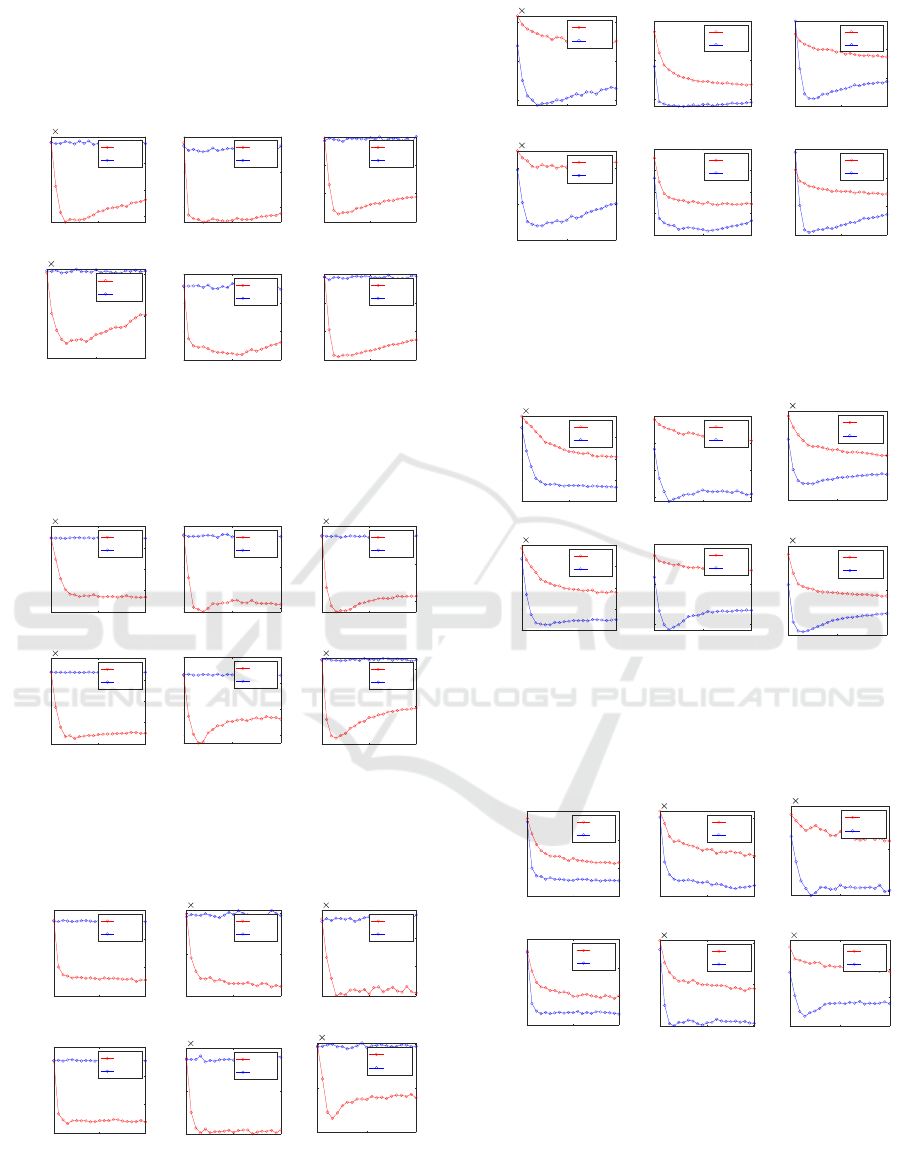
0 0.5 1
PX
3.6
3.65
3.7
3.75
Total Distance
10
4
100 Gens
RWS
TS
0 0.5 1
PX
3.5
3.6
3.7
Total Distance
10
4
200 Gens
RWS
TS
(a) att48
0 0.5 1
PX
450
460
470
480
Total Distance
100 Gens
RWS
TS
0 0.5 1
PX
450
460
470
480
490
Total Distance
200 Gens
RWS
TS
(b) eil51
0 0.5 1
PX
7600
7800
8000
8200
Total Distance
100 Gens
RWS
TS
0 0.5 1
PX
7600
7800
8000
8200
Total Distance
200 Gens
RWS
TS
(c) berlin52
Figure 9: Performance comparison between two selection
strategies (namely, RWS and TS) on TSP instances with
about 50 cities.
0 0.5 1
PX
2.15
2.2
2.25
2.3
2.35
Total Distance
10
4
100 Gens
RWS
TS
0 0.5 1
PX
2.15
2.2
2.25
2.3
2.35
Total Distance
10
4
200 Gens
RWS
TS
(a) kroC100
0 0.5 1
PX
710
720
730
Total Distance
100 Gens
RWS
TS
0 0.5 1
PX
700
710
720
Total Distance
200 Gens
RWS
TS
(b) eil101
0 0.5 1
PX
1.5
1.55
1.6
1.65
Total Distance
10
4
100 Gens
RWS
TS
0 0.5 1
PX
1.5
1.55
1.6
Total Distance
10
4
200 Gens
RWS
TS
(c) lin105
Figure 10: Performance comparison between two selection
strategies (namely, RWS and TS) on TSP instances with
about 100 cities.
0 0.5 1
PX
2550
2600
2650
Total Distance
100 Gens
RWS
TS
0 0.5 1
PX
2500
2550
2600
2650
Total Distance
200 Gens
RWS
TS
(a) rat195
0 0.5 1
PX
1.7
1.75
1.8
Total Distance
10
4
100 Gens
RWS
TS
0 0.5 1
PX
1.7
1.75
1.8
Total Distance
10
4
200 Gens
RWS
TS
(b) d198
0 0.5 1
PX
3.25
3.3
3.35
3.4
3.45
Total Distance
10
4
100 Gens
RWS
TS
0 0.5 1
PX
3.2
3.3
3.4
Total Distance
10
4
200 Gens
RWS
TS
(c) kroA200
Figure 11: Performance comparison between two selection
strategies (namely, RTW and TS) on TSP instances with
about 200 cities.
Besides, this work was supported in part by the Na-
tional Natural Science Foundation of China under
Grant 62006124 and 61873097, in part by the Nat-
ural Science Foundation of Jiangsu under Project
Performance Analysis of Different Operators in Genetic Algorithm for Solving Continuous and Discrete Optimization Problems
543
BK20200811, in part by the Natural Science Founda-
tion of the Jiangshu Higher Education Institutions of
China under Grant 20KJB520006, and in part by the
Startup Foundation for Introducing Talent of NUIST.
0 0.5 1
PX
3.6
3.65
3.7
3.75
Total Distance
10
4
100 Gens
DPiC
SPC
0 0.5 1
PX
3.5
3.6
3.7
Total Distance
10
4
200 Gens
DPiC
SPC
(a) att48
0 0.5 1
PX
460
470
480
Total Distance
100 Gens
DPiC
SPC
0 0.5 1
PX
450
460
470
480
Total Distance
200 Gens
DPiC
SPC
(b) eil51
0 0.5 1
PX
7600
7800
8000
8200
Total Distance
100 Gens
DPiC
SPC
0 0.5 1
PX
7600
7800
8000
8200
Total Distance
200 Gens
DPiC
SPC
(c) berlin52
Figure 12: Performance comparison between two crossover
strategies (namely, DPiC and SPC) on TSP instances with
about 50 cities.
0 0.5 1
PX
2.15
2.2
2.25
2.3
2.35
Total Distance
10
4
100 Gens
DPiC
SPC
0 0.5 1
PX
2.15
2.2
2.25
2.3
2.35
Total Distance
10
4
200 Gens
DPiC
SPC
(a) kroC100
0 0.5 1
PX
710
720
730
Total Distance
100 Gens
DPiC
SPC
0 0.5 1
PX
700
710
720
730
Total Distance
200 Gens
DPiC
SPC
(b) eil101
0 0.5 1
PX
1.55
1.6
1.65
Total Distance
10
4
100 Gens
DPiC
SPC
0 0.5 1
PX
1.5
1.55
1.6
Total Distance
10
4
200 Gens
DPiC
SPC
(c) lin105
Figure 13: Performance comparison between two crossover
strategies (namely, DPiC and SPC) on TSP instances with
about 100 cities.
0 0.5 1
PX
2500
2550
2600
2650
Total Distance
100 Gens
DPiC
SPC
0 0.5 1
PX
2500
2550
2600
2650
Total Distance
200 Gens
DPiC
SPC
(a) rat195
0 0.5 1
PX
1.7
1.75
1.8
Total Distance
10
4
100 Gens
DPiC
SPC
0 0.5 1
PX
1.7
1.75
1.8
Total Distance
10
4
200 Gens
DPiC
SPC
(b) d198
0 0.5 1
PX
3.3
3.35
3.4
3.45
Total Distance
10
4
100 Gens
DPiC
SPC
0 0.5 1
PX
3.2
3.3
3.4
Total Distance
10
4
200 Gens
DPiC
SPC
(c) kroA200
Figure 14: Performance comparison between two crossover
strategies (namely, DPiC and SPC) on TSP instances with
about 200 cities.
0 0.5 1
PX
3.6
3.7
3.8
Total Distance
10
4
100 Gens
SIM
SM
0 0.5 1
PX
3.5
3.6
3.7
Total Distance
10
4
200 Gens
SIM
SM
(a) att48
0 0.5 1
PX
460
480
500
Total Distance
100 Gens
SIM
SM
0 0.5 1
PX
450
460
470
480
490
Total Distance
200 Gens
SIM
SM
(b) eil51
0 0.5 1
PX
7600
7800
8000
8200
Total Distance
100 Gens
SIM
SM
0 0.5 1
PX
7600
7800
8000
8200
Total Distance
200 Gens
SIM
SM
(c) berlin52
Figure 15: Performance comparison between two mutation
strategies (namely, SIM and SM) on TSP instances with
about 50 cities.
0 0.5 1
PX
2.15
2.2
2.25
2.3
2.35
Total Distance
10
4
100 Gens
SIM
SM
0 0.5 1
PX
2.15
2.2
2.25
2.3
2.35
Total Distance
10
4
200 Gens
SIM
SM
(a) kroC100
0 0.5 1
PX
710
720
730
740
Total Distance
100 Gens
SIM
SM
0 0.5 1
PX
700
720
740
Total Distance
200 Gens
SIM
SM
(b) eil101
0 0.5 1
PX
1.5
1.6
1.7
Total Distance
10
4
100 Gens
SIM
SM
0 0.5 1
PX
1.5
1.6
1.7
Total Distance
10
4
200 Gens
SIM
SM
(c) lin105
Figure 16: Performance comparison between two mutation
strategies (namely, SIM and SM) on TSP instances with
about 100 cities.
0 0.5 1
PX
2500
2550
2600
2650
Total Distance
100 Gens
SIM
SM
0 0.5 1
PX
2500
2550
2600
2650
Total Distance
200 Gens
SIM
SM
(a) rat195
0 0.5 1
PX
1.7
1.75
1.8
Total Distance
10
4
100 Gens
SIM
SM
0 0.5 1
PX
1.7
1.75
1.8
Total Distance
10
4
200 Gens
SIM
SM
(b) d198
0 0.5 1
PX
3.3
3.4
3.5
Total Distance
10
4
100 Gens
SIM
SM
0 0.5 1
PX
3.2
3.3
3.4
3.5
Total Distance
10
4
200 Gens
SIM
SM
(c) kroA200
Figure 17: Performance comparison between two mutation
strategies (namely, SIM and SM) on TSP instances with
about 200 cities.
ICEIS 2021 - 23rd International Conference on Enterprise Information Systems
544
(a) f
1
,D = 5 (b) f
2
,D = 5 (c) f
3
,D = 5 (d) f
4
,D = 5
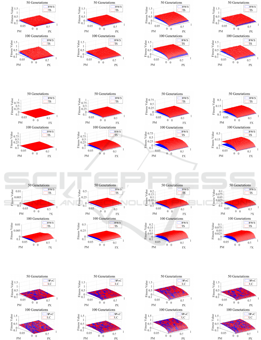
Figure 18: Performance comparison between two selection strategies (namely, RWS and TS) on 5-D NLO functions.
(a) f
1
,D = 15 (b) f
2
,D = 15 (c) f
3
,D = 15 (d) f
4
,D = 15
Figure 19: Performance comparison between two selection strategies (namely, RWS and TS) on 15-D NLO functions.
(a) f
1
,D = 30 (b) f
2
,D = 30 (c) f
3
,D = 30 (d) f
4
,D = 30
Figure 20: Performance comparison between two selection strategies (namely, RWS and TS) on 30-D NLO functions.
(a) f
1
,D = 5 (b) f
2
,D = 5 (c) f
3
,D = 5 (d) f
4
,D = 5
Figure 21: Performance comparison between two crossover strategies (namely, SPoC and UC) on 5-D NLO functions.
Performance Analysis of Different Operators in Genetic Algorithm for Solving Continuous and Discrete Optimization Problems
545

(a) f
1
,D = 15 (b) f
2
,D = 15 (c) f
3
,D = 15 (d) f
4
,D = 15
Figure 22: Performance comparison between two crossover strategies (namely, SPoC and UC) on 15-D NLO functions.
(a) f
1
,D = 30 (b) f
2
,D = 30 (c) f
3
,D = 30 (d) f
4
,D = 30
Figure 23: Performance comparison between two crossover strategies (namely, SPoC and UC) on 30-D NLO functions.
(a) f
1
,D = 5 (b) f
2
,D = 5 (c) f
3
,D = 5 (d) f
4
,D = 5
Figure 24: Performance comparison between two mutation strategies (namely, UM and CM) on 5-D NLO functions.
(a) f
1
,D = 15 (b) f
2
,D = 15 (c) f
3
,D = 15 (d) f
4
,D = 15
Figure 25: Performance comparison between two mutation strategies (namely, UM and CM) on 15-D NLO functions.
ICEIS 2021 - 23rd International Conference on Enterprise Information Systems
546

(a) f
1
,D = 30 (b) f
2
,D = 30 (c) f
3
,D = 30 (d) f
4
,D = 30
Figure 26: Performance comparison between two mutation strategies (namely, UM and CM) on 30-D NLO functions.
REFERENCES
Almunif, A. and Fan, L. (2017). Mixed integer linear
programming and nonlinear programming for optimal
pmu placement. In North Amer. Power Symp., pages
1–6.
Chen, J. C., Cao, M., Zhan, Z. H., Liu, D., and Zhang, J.
(2020). A new and efficient genetic algorithm with
promotion selection operator. In IEEE Trans. Cybern.,
pages 1532–1537.
Eriksen, B. H. and Breivik, M. (2017). Mpc-based mid-
level collision avoidance for asvs using nonlinear pro-
gramming. In Proc. IEEE Conf. Control Technol.
Appl., pages 766–772.
Freisleben, B. and Merz, P. (1996). A genetic local search
algorithm for solving symmetric and asymmetric trav-
eling salesman problems. In Proc. IEEE Int. Conf.
Evol. Comput., pages 616–621.
Ganganath, N., Cheng, C., Fok, K., and Tse, C. K. (2016).
Trajectory planning for 3d printing: A revisit to trav-
eling salesman problem. In Proc. Int. Conf. Control.
Autom. Robot., pages 287–290.
Hildayanti, I. K., Soesanti, I., and Permanasari, A. E.
(2018). Performance comparison of genetic algo-
rithm operator combinations for optimization prob-
lems. In Proc. Int. Seminar Res. Inf. Technol. Intell.
Syst., pages 43–48.
Holland, J. H. (1992). Adaptation in Natural and Artificial
Systems: An Introductory Analysis with Applications
to Biology, Control and Artificial Intelligence. MIT
Press, Cambridge, MA, USA.
Huang, B., Buckley, B., and Kechadi, T.-M. (2010). Multi-
objective feature selection by using nsga-ii for cus-
tomer churn prediction in telecommunications. Expert
Syst. Appl., 37(5):3638 – 3646.
Kaur, D. and Murugappan, M. M. (2008). Performance en-
hancement in solving traveling salesman problem us-
ing hybrid genetic algorithm. In Proc. Biennial Conf.
North Amer. Fuzzy Inform. Process. Soc., pages 1–6.
Li, J., Meng, X., Zhou, M., and Dai, X. (2017). A two-
stage approach to path planning and collision avoid-
ance of multibridge machining systems. IEEE Trans.
Syst. Man Cybern. Syst., 47(7):1039–1049.
Li, Y., Zhang, S., and Zeng, X. (2009). Research of multi-
population agent genetic algorithm for feature selec-
tion. Expert Syst. Appl., 36(9):11570 – 11581.
Ma, F., Xu, Y., and Xu, P. (2017). A nonlinear program-
ming based universal optimization model of tdoa pas-
sive location. In Proc. Int. Conf. Intell. Syst. Knowl.
Eng., pages 1–3.
Pinho, R. and Saraiva, F. (2020). A comparison of crossover
operators in genetic algorithms for switch allocation
problem in power distribution systems. In Proc. IEEE
Congr. Evol. Comput., pages 1–8.
Wang, Z., Fang, X., Li, H., and Jin, H. (2020). An improved
partheno-genetic algorithm with reproduction mecha-
nism for the multiple traveling salesperson problem.
IEEE Access, 8:102607–102615.
Xie, J., Carrillo, L. R. G., and Jin, L. (2019). An inte-
grated traveling salesman and coverage path planning
problem for unmanned aircraft systems. IEEE Control
Syst, 3(1):67–72.
Yang, Q., Chen, W., Gu, T., Zhang, H., Yuan, H., Kwong,
S., and Zhang, J. (2020). A distributed swarm op-
timizer with adaptive communication for large-scale
optimization. IEEE Transactions on Cybernetics,
50(7):3393–3408.
Yang, Q., Chen, W., Li, Y., Chen, C. L. P., Xu, X., and
Zhang, J. (2017a). Multimodal estimation of distribu-
tion algorithms. IEEE Transactions on Cybernetics,
47(3):636–650.
Yang, Q., Chen, W., Yu, Z., Gu, T., Li, Y., Zhang, H., and
Zhang, J. (2017b). Adaptive multimodal continuous
ant colony optimization. IEEE Transactions on Evo-
lutionary Computation, 21(2):191–205.
Yu, F., Fu, X., Li, H., and Dong, G. (2016). Improved
roulette wheel selection-based genetic algorithm for
tsp. In Proc. Int. Conf. Netw. Inf. Syst. Comput., pages
151–154.
Yu, Y., Chen, Y., and Li, T. (2011). A new design of genetic
algorithm for solving tsp. In Proc. Int. Joint Conf.
Comput. Sci. Optim., pages 309–313.
Zhong, J., Hu, X., Zhang, J., and Gu, M. (2005). Compari-
son of performance between different selection strate-
gies on simple genetic algorithms. In Proc. IEEE Int.
Conf. Comput. Intell. Modelling Control Automat. Int.
Conf. Intell. Agents Web Technol. Internet Commerce,
volume 2, pages 1115–1121.
Zhou, H. and Song, M. (2016). An improvement of
partheno-genetic algorithm to solve multiple travel-
ling salesmen problem. In Proc. IEEE/ACIS Int. Conf.
Comput. Inf. Sci., pages 1–6.
Zorlu, O., Dilek, S., and
¨
Ozsoy, A. (2017). Gpu-based par-
allel genetic algorithm for increasing the coverage of
wsns. In Proc. IEEE Int. Conf. Parallel Distrib. Syst.,
pages 640–647.
Performance Analysis of Different Operators in Genetic Algorithm for Solving Continuous and Discrete Optimization Problems
547
