
Feature-based Analysis of the Energy Consumption of Battery Electric
Vehicles
Patrick Petersen, Aya Khdar and Eric Sax
FZI Research Center for Information Technology, Haid-und-Neu-Straße 10-14, 76131 Karlsruhe, Germany
Keywords:
Battery Electric Vehicle, Energy Consumption, Feature Engineering.
Abstract:
Battery electric vehicles have become increasingly important for the reduction of greenhouse gas emission.
Even though the number of battery electric vehicles is increasing, the general acceptance and widespread
introduction to consumers is still related to smaller range, which is in part due to the range anxiety leading to
inefficient usage of the complete battery. Thus, an accurate range estimation is a key parameter for increasing
the trust in the promised range, but accurate estimation is a nontrivial task. Advanced algorithms estimate the
energy consumption based on the travel route and other non-deterministic factors such as driving style, traffic
and weather conditions. The possible feature space is huge, therefore, the identification of a few highly energy
consumption relevant features is necessary due to time and memory limitations in the vehicle including the
improvement of the estimation itself. In this paper we present a data-driven methodology for systematically
analyzing and engineering relevant features which influence the energy consumption concurrently, covering
not only the driver style but also features based on road topology, traffic and weather conditions. Utilizing a
real-world data set different trip segmentation methods and feature selection algorithms are compared to each
other in regards to their accuracy and time-efficiency.
1 INTRODUCTION AND STATE
OF THE ART
Battery electric vehicles (BEVs) are one promis-
ing solution to reduce greenhouse gas emissions and
the dependency on fossil fuels in the mobility sec-
tor (Mahmoudzadeh Andwari et al., 2017). Motivated
by the emission reduction targets (Kodjak, 2015), the
development of efficient BEVs was enforced by vehi-
cle manufactures leading to advances in battery tech-
nology such as capacity and charging performance
as well as the availability of charging points across
the world. However, the perceived limited range of
these vehicles still restrains the adoption of BEVs. In
this context coping with the so called “range anxi-
ety” is the key for the success of BEVs and there-
fore reaching the emission reduction targets. Range
anxiety describes the drivers fear that the electric ve-
hicle does not have sufficient range to reach its des-
tination and therefore being stranded by a depleted
battery is a major concern for the driver (Yuan et al.,
2018). A precise estimation of the available energy
and actually available range, in regards to the route
planned, for increasing the trust in BEVs is essen-
tial. Previous studies on identifying relevant param-
eters in regards to their impact on the energy con-
sumption have mainly focused on investigating driv-
ing patterns, mostly aimed at internal combustion en-
gine vehicles (ICEVs). In the literature driving pat-
terns generally describe the vehicles speed profile and
can be differentiated to driver style or driving behav-
ior (Marina Martinez et al., 2018). As part of the Eu-
ropean ARTEMIS project, a statistical study was per-
formed in order to identify characteristic driving cy-
cles. These were used to develop standardized driv-
ing patterns to test emission and fuel consumption
of ICEVs in a laboratory environment (Boulter and
McCrae, 2007). An analysis of the used parameters
for the characteristic driving cycles identified twelve
driving patterns contrasted in speed, acceleration and
stop rates (Andr
´
e, 2004). Ericsson calculated 62 pa-
rameters to describe driving patterns, which where
then reduced to 16 independent factors by using a
factorial analysis (Ericsson, 2001). A linear regres-
sion was then used to analyze the impact of these
factors for the fuel consumption. Another study in-
vestigated the correlation between driver style and
fuel consumption (Berry, 2010). The results show
that drivers who tend to have an aggressive driver
style have the greatest potential for saving fuel com-
Petersen, P., Khdar, A. and Sax, E.
Feature-based Analysis of the Energy Consumption of Battery Electric Vehicles.
DOI: 10.5220/0010482802230234
In Proceedings of the 7th International Conference on Vehicle Technology and Intelligent Transport Systems (VEHITS 2021), pages 223-234
ISBN: 978-989-758-513-5
Copyright
c
2021 by SCITEPRESS – Science and Technology Publications, Lda. All r ights reserved
223

pared to moderate drivers with lower accelerations.
Driving cycles such as NEDC or WLTP assess the
emission levels of car engines and their fuel or en-
ergy consumption (Sileghem et al., 2014). However,
they don’t reflect real usage of a vehicle due to the
laboratory design of these driving cycles (Fontaras
et al., 2017). Therefore, investigating the consump-
tion under real-world driving conditions is essential.
Similar to fuel consumption, the energy consump-
tion of BEVs correlates with the driver style, this im-
plies that the energy efficiency of BEVs has a posi-
tive correlation with the average speed of the given
route (Knowles et al., 2012). Younes et al. fur-
ther investigated the energy consumption during dif-
ferent real-world driving conditions (such as tempera-
ture, routes, driver style) (Younes et al., 2013). It was
shown that the energy consumption relates to driving
parameters covering velocity and acceleration. Addi-
tionally, they point out that driving parameters can be
used for differentiating between types of routes and
driver styles. However, the results demonstrate that
a single driving parameter can not distinguish both
the driver style and the route type at once. Badin et
al. evaluated the impact of influencing factors such as
driving conditions, driver’s aggressiveness and the us-
age of auxiliaries via correlation (Badin et al., 2013).
De Cauwer et al. used multiple physical models to de-
tect and quantify the correlation between kinetic vehi-
cle parameters and energy consumption (De Cauwer
et al., 2015). Braun and Rid investigated whether
driving patters designed for the fuel consumption of
ICEVs are also relevant for the energy consumption
of BEVs (Braun and Rid, 2018). They provide an
in-depth analysis of 45 driving parameters and their
correlation to the energy consumption. Followed by
applying an exploratory factor analysis to reduce the
existing set of parameters to 6 independent driving
pattern factors. Their results show that the intensity
of acceleration and deceleration have the most sig-
nificant correlation with the energy consumption. Si-
monis and Sennefelder developed a data-based range
estimating model based on driver-specific parame-
ters (Simonis and Sennefelder, 2019). By applying
a correlation analysis they selected suitable parame-
ters for their model, allowing an accurate estimating
of the future energy consumption. In all the studies
reviewed here, driving patterns are recognized as a
main influence on the energy consumption of BEVs.
However, the defined driving patterns are strongly in-
fluenced by external factors such as road topology,
traffic and weather conditions (Huang et al., 2011).
Factors found to be influencing the energy consump-
tion of BEVs have been explored in several studies.
Si et al. clustered and evaluated a set of driving pat-
terns together with route information (such as road
type and slope) (Si et al., 2018). Their results show
that the surrounding conditions have a significant in-
fluence on the driver style. Furthermore, they point
out that driving patterns can vary from one driving
circumstance to another. Drivers tend to change their
driver style regardless of the driving condition. An-
other study demonstrated that the aggressiveness of
a driver has a distinctive influence on the fuel con-
sumption for different road grades (Faria et al., 2019).
They found out that for aggressive drivers lower road
grades tend to correlate with a higher increase on fuel
consumption. Yi and Bauer provide a stochastic sen-
sitivity analysis of energy consumption and four en-
vironmental variables (such as wind speed and tem-
perature). The results show a drastic effect on the
energy consumption (Yi and Bauer, 2017). The data-
driven machine learning model by De Cauwer et al.
uses additional geographical and weather data to es-
timate the energy consumption for a given route (De
Cauwer et al., 2017). Smuts et al. name 44 factors
which influence the driving range and introduce a tax-
onomy of factors which are covering the road (such
as road topology and traffic regulations), the terrain
(such as elevation and slope), the driver style (such as
driving speed and trip distance), environmental con-
ditions (such as temperature and wind speed) as well
as vehicle modeling (such as mass and traction) and
the battery modeling (such as state of charge and bat-
tery temperature) (Smuts et al., 2017). They note that
most of the state-of-the-art algorithms only cover an
average of 40 % of the factors for their estimations.
Therefore, an accurate algorithm should incorporate
parameters covering all of the identified influencing
factors. However, the resulting feature space could be
too large leading to the well known ”Curse of dimen-
sionality”, by over fitting the model (Bellman, 2015).
Decreasing the high dimensional feature space, by
removing less important features, is a common ap-
proach to cope with it (Verleysen and Franc¸ois, 2005).
This needs to be done without loosing relevant infor-
mation for the model. Despite this interest, no one to
the best of our knowledge has studied a feature based
analysis of driving patterns concurrently together with
the calculation for other influencing factors such as
road topology, weather and traffic conditions. Thus,
this paper aims to extend the mentioned related work
by presenting a study, based on real-world driving
data, which examines the influences for the energy
consumption not only by calculating driver style pa-
rameters but also for calculating parameters covering
other factors such as road topology, weather and traf-
fic conditions concurrently. In addition different seg-
mentation methods for feature engineering as well as
VEHITS 2021 - 7th International Conference on Vehicle Technology and Intelligent Transport Systems
224
different feature selection methods are compared to
each other. The remaining sections of this work are
structured as follows: Section 2 provides the method-
ology for developing relevant features for the energy
consumption of BEVs. This is done by designing the
parameters for each influencing factor, choosing the
data segmentation method as well as comparing dif-
ferent feature reduction methods in regards to their
variance and time. Additionally, the data acquisition
for the analysis is presented. In Section 3 the real-
world data pool for the experimental implementation
is presented. Based on the availability and quality
of data respective features are calculated, proposed
methods for the reduction of feature-space are eval-
uated and compared to each other. Finally, Section 4
concludes the paper and discusses future work based
on the results.
2 METHODOLOGY FOR
FEATURE-BASED ANALYSIS
OF THE ENERGY
CONSUMPTION
Due to the importance of selecting relevant fea-
tures for the energy consumption it is not feasi-
ble to manually select them, therefore, a automated
data-driven approach is necessary. Our goal was
to create a methodology, which enables an exhaus-
tive analysis of the most relevant features for the en-
ergy consumption based on real-world driving data.
Therefore, our methodology is inspired by similar
processes like Knowledge Discovery in Databases
(KDD) and Cross-industry standard process for data
mining (CRISP-DM) for extracting knowledge from
our databases. The KDD process consists of nine
steps, which can be generally summarized to five
steps: data selection, data preprocessing, transfor-
mation, data mining and interpretation (or evalua-
tion) (Kawano, 1997). The CRISP-DM process de-
fines the steps as follows: business understanding,
data understanding, data preparation, modeling, eval-
uation and deployment (Shearer et al., 2000). In
compliance with the two established data mining pro-
cesses we consider a simplified process consisting of
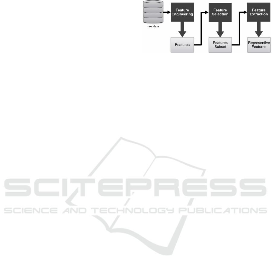
three main steps, which are shown in Figure 1. The
methodology starts with the so called feature engi-
neering, which describes the process of preparing the
raw data in such a way that it can be used for the ex-
traction of features. In the feature selection step the
most relevant subset of features for the energy con-
sumption are identified. In the final feature extrac-
tion step, the identified subset of relevant features will
Figure 1: Overview of the main steps of the methodology.
be reduced via dimensionality reduction techniques to
reduce redundant data for the analysis.
2.1 Feature Engineering
Feature engineering covers all processing steps so that
the original raw data can be used directly by machine
learning algorithms. The idea is that feature engineer-
ing creates a better starting point for machine learning
models by providing correct, relevant and meaningful
data representation. It covers the preprocessing step
of smoothing noise, methods of segmenting data in
suitable and meaningful parts as well as transforming
raw data into aggregated features.
2.1.1 Data Smoothing
Real-world data is recorded as time series and suitable
signal preprocessing is required due to signal noise
and errors. In general, noisy data can have negative
impact on the performance and the accuracy of a ma-
chine learning model (Zhu and Wu, 2004). Hence,
smoothing the raw signals can be a suitable way, de-
pending on the signal and its encoded information, to
cope with this noise. This is done via smoothing fil-
ters which replace values of a time series with new
values obtained from e.g. local averages of surround-
ing values. These filters have the benefit of remov-
ing noise in time series without distorting the sig-
nal tendency. In this research we use the Savitzky-
Golay (SG) filter, originally published in 1964 (Sav-
itzky and Golay, 1964). In contrast to other low-pass
filter, which are applied in the frequency domain, the
SG filter is applied in the time domain. The main idea
of the SG filter is to apply for each data point a least-
square fit with a polynomial p of order n within an
odd-sized window of length N = 2M + 1 centered at
the reconstruction point of the signal, where M rep-
resents the number of neighboring points on the left
and the right side (Schafer, 2011). The defined poly-
nomial p with order n is then fitted to the samples N
of the noisy signal f to minimize the squared approx-
imation error ε
n
defined as follows:
ε
n
=
M
∑
i=−M
(p(i) − f (i))
2
Feature-based Analysis of the Energy Consumption of Battery Electric Vehicles
225

2.1.2 Segmentation Methods
For the feature analysis of real-world driving data it
is important to pay particular attention to the gran-
ularity of the developed features. Calculating fea-
tures on a complete trip may remove fine-grained im-
portant information such as sudden changes in the
velocity profile due to specific traffic or road topo-
logical conditions. Thus, recorded data should be
segmented in such a way that calculated features
still contain enough fine-grained information. Sev-
eral studies applied different segmentation methods,
which can be categorized into static and dynamic seg-
mentation methods. Figure 2 shows the recording of
Controller Area Network (CAN) data of a trip includ-
ing an exemplary segment for the segmentation ap-
proaches. Static segmentation uses a fixed interval
Figure 2: Illustration of the resulting segments using time-
based static segmentation, grouping variables and micro-
trips on real-world driving data.
(e.g. distance or time) to segment data into smaller
parts. Thus, all segments have the same length in time
or distance. De Cauwer et al. used static time inter-
val of length of 2 min, 5 min, and 10 min to segment
trips for training a model to predict the energy con-
sumption (De Cauwer et al., 2015). Another study
further investigated the effects of different data seg-
mentation methods for the modeling of vehicle en-
ergy consumption (Li et al., 2017). They mention that
such static segmentation methods may cause disconti-
nuities to some information such as traffic. Due to the
nature of that method it is difficult to aggregate cate-
gorical information into one feature such as changing
speed limits within such static segments. Dynamic
segmentation relies on different signal curves for seg-
menting a trip. Two common approaches exist for the
dynamic segmentation. One is the segmentation into
micro-trips. They utilize the velocity profile to seg-
ment a trip into sequences between two stops. Thus,
micro-trips include acceleration, cruising and decel-
eration of the vehicle (Kamble et al., 2009), but they
also suffer from discontinuities as well as the afore-
mentioned aggregation of information to one features
for a segment. Also the length of a micro-trip can vary
a lot due to the frequency of stops along a trip. If the
vehicle does only stop at the end of the trip the whole
trip will be used as a segment and therefore may lose
fine-grained information. The other approach for dy-
namic segmentation is grouping variables. They use
variables such as street type or speed limit for the
segmentation. A trip is divided when the value of at
least one selected variable is changing. This ensures
homogeneous static information for the used group-
ing variable and makes the aggregation of features
easier. Popular representatives of this approach are
data providers such as Google or HERE. They use
a link-based segmentation for their navigation sys-
tems. Links are acquired via a defined set of grouping
variables (HERE, 2021) (Google, 2021). Ericson et
al. used 11 grouping variables related to street, ve-
hicle, traffic and driver to segment their data (Erics-
son, 2001). Langner et al. use categorical and or-
dinal signals for separating scenarios within the test
drives (Langner et al., 2019)
2.1.3 Transformation of Raw Data
Selecting the correct representation of data for fea-
tures is one of the most important steps in the engi-
neering process. Transforming and aggregating raw
data into suitable features is nontrivial and often re-
quires a lot of time when done manually. Typically
domain knowledge from an expert is used for the en-
gineering of features and therefore it can be a tedious
task. Experts engineer features by aggregating, trans-
forming and calculating raw data to new semantic fea-
tures. By relying on an expert, engineering features
can be limited by human subjectivity as well as time
constraints. However, automated feature engineer-
ing tools and libraries (such as tsfresh (Christ et al.,
2018)) exist to cope with this problem by automati-
cally calculating hundreds of new statistical features
on the given dataset. As mentioned in the introduction
of this paper (see Section 1) features should cover the
energy consumption relevant categories such as driv-
ing style, street topology, traffic and environmental
conditions. Table 1 illustrates the researched litera-
ture and gives a brief overview of the general covered
features of this study. The table shows the relevant
papers in which the features were originally intro-
duced. Some of them describe statistics such as mean,
median and standard derivation of raw data such as
speed, acceleration, elevation and slope. Other fea-
tures are rule-based for example the aggressiveness of
a driver is based on multiple conditions depending on
the acceleration, speed and frequency of pedal-usage.
VEHITS 2021 - 7th International Conference on Vehicle Technology and Intelligent Transport Systems
226

Table 1: Overview of the energy consumption relevant features for driving style, street topology, traffic and environmental
conditions.
Feature Categories References
Driving Style
Speed
(Ericsson, 2001), (Braun and Rid, 2018), (Grubwinkler et al., 2014), (Si et al., 2018),
(Grubwinkler et al., 2013), (Larsson and Ericsson, 2009), (Diaz Alvarez et al., 2014)
Acceleration
(Ericsson, 2001), (Braun and Rid, 2018), (De Cauwer et al., 2015), (Si et al., 2018),
(Grubwinkler et al., 2013), (Diaz Alvarez et al., 2014)
Aerodynamic work
(Ericsson, 2001), (Braun and Rid, 2018), (De Cauwer et al., 2015)
Positive/Negative kinetic energy
(Ericsson, 2001), (Braun and Rid, 2018)
Oscillation in speed profile
(Ericsson, 2001), (Braun and Rid, 2018)
Aggressiveness features
(Badin et al., 2013), (Jasinski and Baldo, 2017), (Birrell et al., 2014), (Filev et al., 2009)
Jerk
(Murphey et al., 2009), (Si et al., 2018), (Diaz Alvarez et al., 2014)
Topology
Slope
(Smuts et al., 2017), (Faria et al., 2019), (Si et al., 2018)
Elevation
(Iora and Tribioli, 2019), (De Cauwer et al., 2015), (Grubwinkler et al., 2013), (Wittmann et al., 2018)
Curvature
(Grubwinkler et al., 2013)
Curviness
(Wittmann et al., 2018), (Langner et al., 2019)
Traffic
Jam time
(Xue et al., 2014), (Loulizi et al., 2019)
Free flow
(Xue et al., 2014)
Street class
(Faria et al., 2019), (Wang et al., 2018)
Stop time
(Braun and Rid, 2018)
Environment
Temperature features
(Iora and Tribioli, 2019), (Smuts et al., 2017), (Li et al., 2016)
Daylight
(Grubwinkler et al., 2014)
Sun Altitude, Radiation, Intensity
(Birrell et al., 2014), (Pysolar, 2021)
Air conditioner usage
(De Cauwer et al., 2015), (Liu et al., 2017)
Power of auxiliaries
(De Cauwer et al., 2015), (Liu et al., 2017)
2.2 Feature Selection
The risk of overfitting as well as the curse of dimen-
sionality can be caused by a large number of features.
Furthermore, training time of a model increases ex-
ponentially with the number of features (Aggarwal
et al., 2014). Thus, the utilization of feature selec-
tion algorithms is essential. Feature selection is the
process of selecting the most relevant features to the
energy consumption of BEVs and discarding the ir-
relevant features. Feature selection processes increase
accuracy, reduce overfitting and training time for ma-
chine learning models by evaluating the importance of
features and selecting only a relevant subset that im-
proves the accuracy of the model. Feature selection
algorithms can be divided into filter, wrapper and em-
bedded approaches (Chandrashekar and Sahin, 2014)
(Guyon and Elisseeff, 2006).
2.2.1 Filter
Filter methods select relevant features independently
of a machine learning model. They evaluate the im-
portance of features by relying on the general charac-
teristics of the data itself such as statistical dependen-
cies or distances between classes (Bosin et al., 2007).
As the name suggests they filter out features before
a machine learning model is trained. A popular filter
method is a correlation-based approach, which selects
features that correlate with the target feature and mini-
mize redundant features in the feature set. Depending
on the feature (continuous and categorical) an appro-
priate correlation needs to be applied. Correlation-
based approaches have low intercorrelation (Khalid
et al., 2014), which means just one of the features
with collinearity should be selected to remove addi-
tional redundancy. Due to the ease of filter methods
their main characteristic are their speed and scalabil-
ity.
2.2.2 Wrapper
Wrapper methods evaluate the impact of different
subsets of features using a machine learning model
(e.g. a predictive model) by calculating the estima-
tion accuracy of each feature subset separately (Ag-
garwal et al., 2014). Those methods can be catego-
rized as greedy algorithms due to their strategy to
find the best possible subset. Thus, they can result
in a computationally expensive search. The wrapper
selection is performed gradually by applying differ-
ent search strategies for the feature selection such as
genetic algorithms, random search and sequential se-
lection search (Rodriguez-Galiano et al., 2018) (El
Aboudi and Benhlima, 2016). In the following three
common wrapper method implementations are intro-
duced:
Sequential Backward Selection. The sequential
backward selection (SBS) is one of the first devel-
oped methods of the wrapper family (Shen, 2009).
Starting with the whole feature set it gradually tries
Feature-based Analysis of the Energy Consumption of Battery Electric Vehicles
227

to eliminate the least relevant feature by using a ma-
chine learning model to evaluate the remaining fea-
ture subsets (Guyon et al., 2006). The elimination
process stops when all the remaining features meet
the criterion of the model e.g. the a priori desired
number of remaining features. SBS does not guaran-
tee to find the optimal solution, but it is ensured to
converge quickly. Thus, choosing the right criterion
for the model is critical to result in a near optimal so-
lution.
Sequential Forward Selection. The sequential for-
ward selection (SFS) is one of the simplest greedy
search algorithms. This method performs a forward
selection by gradually adding features to feature sub-
sets and evaluating them (Marcano-Cede
˜
no et al.,
2010). In every iteration a machine learning model is
used to evaluate the feature subset by calculating the
model accuracy of the subset. The feature subset with
the best result is then selected. The selection process
stops when the a priori predefined number of features
is selected. However, SFS may suffer from obsolete
features being added to the subset, if the number of
features is to high or missing relevant features, when
the number is to low (Chandra, 2015).
Recursive Feature Elimination. The Recursive
Feature Elimination (RFE) is the opposite approach
to forward selection (Le Thi et al., 2008). It starts
with all features to train a machine learning model
and gradually build smaller feature subsets. The algo-
rithm continues with the subset with the best features
until the specified number of features is reached (Le
Thi et al., 2008). Unlike SBS it does the whole elim-
ination cycle and then chooses the best subset instead
of stopping when the criterion for the model is met.
2.2.3 Embedded
In contrast to filter or wrapper methods, embedded
methods integrate feature selection in the machine
learning model (e.g. classifier). Embedded methods
select features that contribute the most to the accuracy
of the model when the model is being created (Aggar-
wal et al., 2014). The embedded model performs fea-
ture selection during training. In other words, it per-
forms model fitting and feature selection simultane-
ously (Lal et al., 2006). Thus, it is less prone to over-
fitting and can be more accurate than filter methods
due to directly selecting feature subsets for the trained
algorithm. The embedded methods include the Least
Absolute Shrinkage and Selection Operator (LASSO)
method (Fonti, 2017). LASSO aims to minimize the
prediction error using two main steps: regularization
and feature selection. During the regularization step
it shrinks the coefficient of the regression variables to
reduce the risk of overfitting. Then, during the feature
selection step features that still have a non-zero coef-
ficient are selected, which results in a good prediction
accuracy (Fonti, 2017). It involves a penalty factor,
which determines the correct number of features.
2.3 Feature Extraction
Feature selection methods aim to find the most rele-
vant feature subset for a defined target feature (in this
work the energy consumption). However, the num-
ber of selected features can still be to big. Thus, to
increase the accuracy and the efficiency of a machine
learning model, it is recommended to apply additional
dimension reduction methods (Prabhu, 2011). By ap-
plying feature extraction the selected subset of fea-
tures is transformed into a lower dimensional space
resulting in fewer previously selected features. Pop-
ular examples of dimension reduction methods are
Principal Component Analysis (PCA) or exploratory
factor analysis (EFA). PCA analyzes the total vari-
ance in the data set, whereas EFA depends on a com-
mon factor model, which assumes that the observed
variance in features is attributed to a single specific
factor (Anand et al., 2014). EFA reduces a large space
of features by producing a lower space of factors,
whereas each factor includes the strongly correlated
features. EFA uses variances to find the commonal-
ities between features, that is described by the sum-
mation of the squared correlation of the feature with
the factors (Yong and Pearce, 2013). There are differ-
ent methods to select the suitable number of factors
using extracted variance and eigenvalue, which de-
scribes the amount of the variance in the data that can
be explained by the associated factor (Beavers et al.,
2013a). The Kaiser criterion suggests retaining all
factors that have eigenvalues greater than one (Yong
and Pearce, 2013).
3 RESULTS AND DISCUSSION
In this research, data was collected from different test
drives in Germany, Austria and USA in the years 2018
to 2019. The recorded real-world data was collected
from different drivers and routes over several months.
Table 2 provides an overview of the data. The data
contains recorded signals from the CAN mainly cov-
ering vehicle-centric operation states in a time-based
format. All signals on the CAN are sampled with dif-
ferent frequencies up to 50 Hz and more. We decided
to sample the data at 10 Hz to still represent relevant
VEHITS 2021 - 7th International Conference on Vehicle Technology and Intelligent Transport Systems
228

Table 2: Overview of the used data for the evaluation.
Vehicle Porsche Taycan
Number of trips 234
Total length 8878 km
Shortest trip 12.64 km
Longest trip 156.75 km
Average length 54.38 km
Quota urban 37 %
Average velocity 71.43 km/h
driver styles and road characteristics. The recorded
signals consist of a timestamp, GPS position, vehicle
speed, vehicle longitudinal and lateral acceleration as
well as current slope and the total electrical power
(supply for traction battery and generative braking).
For smoothing noisy real-world data the SG filter was
applied. To further increase data quality and variety
of the recorded CAN we extracted additional informa-
tion from data providers, due to their relevance for the
energy consumption and range estimation of BEVs.
Historical traffic data was obtained from the data
provider HERE by matching historical traffic speed
to time and date of departure for each recorded test
drive. Information about the weather condition during
the trip were limited on recorded CAN alone due to
additional information about historical weather con-
ditions from data providers were not available during
the experiment. The free and open source databases
Meteostat
1
did not offer enough relevant historical
weather data for the recorded trips to be used in this
research. For the granularity of feature engineer-
ing we investigated the aforementioned segmentation
methods on our data. Depending on the length of
static segmentation it results in inhomogeneous fea-
tures for a segment such as categorical features e.g.
speed limit and street class are, therefore, not usable
for aggregation and not suitable for the feature engi-
neering. While smaller intervals may solve this issue,
the semantic meaning of each segment as well as the
aggregation of similar test content may get lost in the
process. Micro-trip segmentation results in very long
segments due to most of the recorded trips did not
include enough stops resulting into segments cover-
ing the whole recorded trip. By applying grouping
variables (speed limit and street class) the segments
resulted into suitable segments including enough data
points for the calculation of features as well as of-
fering homogeneous data for the aggregation of cat-
egorical features which where analyzed in this study.
In addition, this approach fits the routing concept of
Google or HERE and is the basis for state-of-the-
art range estimation algorithms. The mean length of
1
Meteostat website: https://meteostat.net
a segment was about 120 m leading to 74,000 data
points, which is enough data for the investigation.
Based on the literature research in Table 1 features
were selected in accordance to their availability in the
data pool as well as their raw data quality. A total
of 105 features were chosen and calculated on each
segment covering driver style, road topology, weather
and traffic conditions. They mainly consist of statis-
tical measures such as average, median and standard
derivation of respective signals such as speed, slope or
curvature. For the driver style some of them consist
of a rule-based approach for identifying an aggressive
or calm driver style.
For selecting the most relevant subset of features,
five feature selection methods were implemented and
their performance were evaluated by applying the R
2
scoring metric on each subset (Anderson-Sprecher,
1994). The features in this work include both contin-
uous and discrete ordinal features. Thus, Spearman
correlation is utilized for the correlation-based filter
method because it is a suitable method to handle or-
dinal variables (Thirumalai and Member, 2017). It
analyses the relationships between the ranks of fea-
tures instead of their value. Table 3 shows the num-
ber of selected features of the subset, its accuracy and
the execution time of each feature selection method.
The execution time is measured on a PC with an In-
Table 3: Comparison of feature selection methods in re-
gards to their R
2
score and execution time.
Method # Features R
2
R
2
R
2
Time [s]
Filter 19 0.95 17.42
SBS 56 0.95 2.05
SFS 30 0.97 45.14
RFE 30 0.95 18.21
LASSO 43 0.97 0.77
tel Core i7 processor which runs at a frequency of
3.20 GHz. Overall, the implemented feature selection
methods have an R
2
between 0.95 and 0.97. They
mainly differ in their selected number of features and
execution time. SFS and LASSO return the best R
2
score while LASSO takes the least amount of time
for execution but still include the second most num-
ber of features in its final feature subset. The filter
method offers the best trade-off in regard to selected
number of features, R
2
and execution time. However,
all implemented methods still retain a high number
of features, thus the feature extraction step for addi-
tional dimension reduction is necessary. To further
reduce the number of features EFA is applied for the
feature extraction. In this work, Kaiser’s criterion is
implemented to find the number of factors to retain
Feature-based Analysis of the Energy Consumption of Battery Electric Vehicles
229

Figure 3: A sample scree plot for the features of the RFE
feature selection method.
which have eigenvalues greater than one. Figure 3
shows a scree plot for the Kaiser’s criterion applied
on the 30 selected factors using RFE. 9 factors have
eigenvalues ≥ 1 and thereby meet the Kaiser’s crite-
rion. The percentage of data that could be predicted
using the selected number of factors is known as ex-
tracted variance. For the factors from the selected
feature subsets, the variance is calculated for compar-
ison. The threshold for sufficient extraction of fac-
tors is suggested to be between 75 % - 90 % (Beavers
et al., 2013a). Table 4 compares the resulting factors
and corresponding extracted variances for the feature
subset from feature selection methods. Based on the
Table 4: Comparison of the extracted variance and the cor-
responding number of factors of each selected feature sub-
set of feature selection methods.
Method Features Factors Variance
Filter 19 5 0.56
SBS 56 18 0.69
SFS 30 9 0.63
RFE 30 9 0.80
LASSO 43 18 0.65
results in Table 4 feature extraction performed on the
feature subset using RFE has the highest variance of
0.80 compared to the others. The extracted factors
from RFE are 9 in total. The lowest number of fac-
tors, 5 in total, can be extracted from the filter method
but the resulting variance of 0.56 is the lowest of them
all. The variance of the 9 factors from RFE meets the
criterion of ≥ 0.75 thus they are to be preferred. Fig-
ure 4 shows the percentage of data that is explained
with each individual factor and the cumulative vari-
ance (80 %) of the 9 extracted factors. For better inter-
pretation of the factors it is common to apply rotation
methods to reduce ambiguity. Rotation methods try to
distribute the feature load to as few factors as possi-
ble, thus, maximize the number of high loads on each
Figure 4: Explained variance of each extracted factor and
its cumulative variance.
variable. Hence, factors can be easier interpreted due
to fewer associated features. For rotation there exist
two common approaches: orthogonal and oblique ro-
tation (Yong and Pearce, 2013). In this work Varimax
rotation is use to minimize the number of features that
have high loading on each factor. It belongs to the or-
thogonal rotations which rotate factors 90
◦
from each
other. Figure 5 shows the factor loadings after rotation
using Varimax method. Each column represents the
extracted factors and its corresponding factor loading
after the Varimax rotation. Each factor describes a
certain category of features e.g. the 5th factor can
be expressed as an topology feature like mean slope.
Each factor includes strong correlated features with
each others, thus, it is sufficient to select the most
representative feature from each factor. A feature is
in general considered as a good representative of the
factor if its absolute loading ≥ 0.70 and if it does have
a high intersecting loading on another factor (Beavers
et al., 2013b). The study (Guo et al., 2002) suggests
to select one or a few representative features with the
absolute largest loading to keep as much variance as
possible. As a result, the final subset includes the 9
most representative features. Table 5 shows the final
subset of features. An initial objective of this study
Table 5: Representative features: from each factor, one of
the good identifier feature is selected, which has a absolute
loading ≥ 0.70.
Nr. Category Feature
1 Driver Style Time Weighted Mean Acceleration
2 Traffic % of Speed < 2 km/h
3 Driver style & Traffic Averaged Squared Speed
4 Driver style % of Deceleration 0.0 m/s
2
- 0.5 m/s
2
5 Street topology Mean Slope
6 Driver Style Time Weighted Mean Decelerating
7 Environment (Weather) % of Nightlight
8 Driver style & Traffic % of Speed 50 km/h - 100 km/h
9 Driver style & Traffic % Deceleration 1.0 m/s
2
- 1.5 m/s
2
was to identify suitable feature engineering steps cov-
ering engineering, selection and extraction methods
VEHITS 2021 - 7th International Conference on Vehicle Technology and Intelligent Transport Systems
230
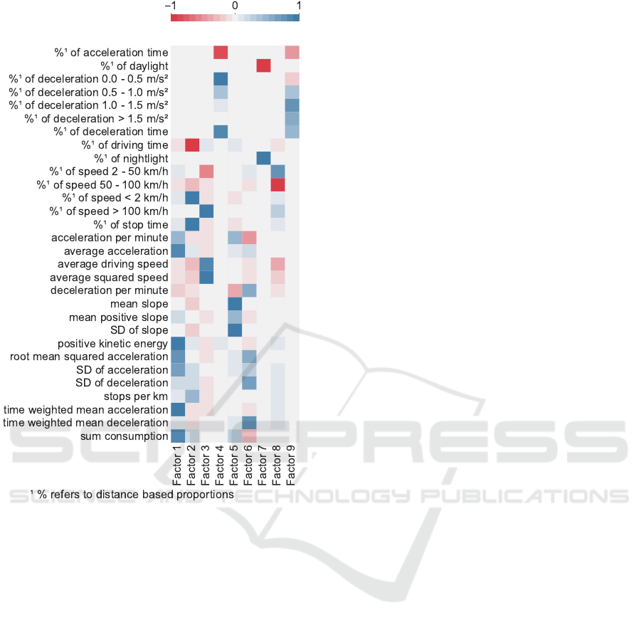
Figure 5: Factor loadings matrix describing the correlation
between the features and the extracted factor.
for the analysis of energy consumption relevant fea-
tures. As mentioned in the literature review, different
categories such as driving style, traffic and weather
conditions need to be considered when selecting rele-
vant features for the energy consumption. The results
of this study did show that the previously calculated
105 features can be reduced to a final subset of 9 sig-
nificant features for the energy consumption covering
the aforementioned categories and 80 % of the orig-
inal data’s variance. This finding has important im-
plications for developing range estimation algorithms
and the features which should be taken into account
for an accurate estimation. This could not be done on
driving cycles such as WLTP due to their laboratory
design, which does not cover the influence of traffic
or weather conditions.
4 CONCLUSION AND FUTURE
WORK
This paper presented a methodology for a data-driven
analysis of energy relevant factors covering driver
style, weather conditions, road topology and traffic
parameters. The methodology consists of three main
steps: feature engineering, feature selection and fea-
ture extraction. Feature engineering converts raw
data into features on homogeneous segments of the
trips. Based on real-world data different segmentation
methods such as static and dynamic approaches were
introduced and compared to each other. Segmenta-
tion based on speed limit and street type as group-
ing variables had the best trade off between ease of
use, flexibility and sufficient length for the feature en-
gineering step. For each segment different features
were calculated for the influencing factors leading to
a total of 105 features. During the feature selection
step the most relevant subset of features to the energy
consumption were selected. By comparing different
feature selection methods in regards to their accuracy
of the R
2
score, the calculation time and the resulting
number of selected features we chose the RFE method
as the promising technique. Resulting in 30 features
in total. By utilizing feature extraction via EFA we
identified the underlying relationship between the se-
lected features to reduce dimension and specified the
most representative 9 features. These 9 features cover
80 % of the original data’s variance.
We have shown that our concept allows to select
and reduce relevant features for the energy consump-
tion of BEVs under real-world conditions. Covering
not only driver style features but also concurrently
investigating features for road topology, traffic and
weather conditions. By selecting relevant features via
a data-driven approach a biased feature selection from
experts can be avoided.
Future work will focus on increasing the amount
of data in terms of number and variety to improve the
robustness of the proposed methodology and the cur-
rent results. Covering additional drivers, countries,
weather conditions, vehicle models and in general dif-
ferent driving situations. The right amount of data
needed for an exhaustive analysis while keeping the
experiment time and cost low needs to be addressed
as well. In addition, applying automated feature en-
gineering tools or libraries to emphasize a fully au-
tomated data-driven feature-based analysis of the en-
ergy consumption of BEVs will be investigated.
Integrating the extracted relevant features, for the
energy consumption, into state-of-the-art range esti-
mation algorithms to further investigate and validate
the benefits of our proposed methodology will be in-
Feature-based Analysis of the Energy Consumption of Battery Electric Vehicles
231

vestigated as well.
ACKNOWLEDGEMENTS
We would like to thank Dr. Ing. h.c. F. Porsche AG for
providing the data for this study.
REFERENCES
Aggarwal, C. C., Kong, X., Gu, Q., Han, J., and Yu, P. S.
(2014). Active learning: A survey. Data Classifica-
tion: Algorithms and Applications, pages 571–605.
Anand, S., Padmanabham, P., and Govardhan, A. (2014).
Application of Factor Analysis to k-means Cluster-
ing Algorithm on Transportation Data. International
Journal of Computer Applications, 95(15):40–46.
Anderson-Sprecher, R. (1994). Model comparisons and R
2. The American Statistician, 48(2):113–117.
Andr
´
e, M. (2004). The ARTEMIS European driving cycles
for measuring car pollutant emissions. Science of the
Total Environment, 334-335:73–84.
Badin, F., Le Berr, F., Briki, H., Dabadie, J. C., Petit,
M., Magand, S., and Condemine, E. (2013). Evalua-
tion of EVs energy consumption influencing factors:
Driving conditions, auxiliaries use, driver’s aggres-
siveness. World Electric Vehicle Journal, 6(1):112–
123.
Beavers, A. S., Lounsbury, J. W., Richards, J. K., Huck,
S. W., Skolits, G. J., and Esquivel, S. L. (2013a).
Practical Considerations for Using Exploratory Factor
Analysis. 18(6).
Beavers, A. S., Lounsbury, J. W., Richards, J. K., Huck,
S. W., Skolits, G. J., and Esquivel, S. L. (2013b). Prac-
tical considerations for using exploratory factor analy-
sis in educational research. Practical Assessment, Re-
search and Evaluation, 18(6):1–13.
Bellman, R. (2015). Adaptive Control Processes - {A}
Guided Tour (Reprint from 1961), volume 2045 of
Princeton Legacy Library. Princeton University Press.
Berry, I. M. (2010). The Effects of Driving Style and Vehicle
Performance on the Real-World Fuel Consumption of
US Light-Duty Vehicles. PhD thesis, Massachusetts
Institute of Technology.
Birrell, S. A., McGordon, A., and Jennings, P. A. (2014).
Defining the accuracy of real-world range estima-
tions of an electric vehicle. 2014 17th IEEE Interna-
tional Conference on Intelligent Transportation Sys-
tems, ITSC 2014, pages 2590–2595.
Bosin, A., Dess
`
ı, N., and Pes, B. (2007). Intelligent Data
Engineering and Automated Learning - IDEAL 2007.
Ideal, 4881(December):790–799.
Boulter, P. G. and McCrae, I. S. (2007). ARTEMIS: Assess-
ment and Reliability of Transport Emission Models
and Inventory Systems-Final Report. TRL Published
Project Report.
Braun, A. and Rid, W. (2018). Assessing driving pattern
factors for the specific energy use of electric vehicles:
A factor analysis approach from case study data of the
Mitsubishi i–MiEV minicar. Transportation Research
Part D: Transport and Environment, 58(2018):225–
238.
Chandra, B. (2015). Gene Selection Methods for Microar-
ray Data. Elsevier Inc.
Chandrashekar, G. and Sahin, F. (2014). A survey on fea-
ture selection methods. Computers and Electrical En-
gineering, 40(1):16–28.
Christ, M., Braun, N., Neuffer, J., and Kempa-Liehr, A. W.
(2018). Time Series FeatuRe Extraction on basis of
Scalable Hypothesis tests (tsfresh – A Python pack-
age). Neurocomputing, 307:72–77.
De Cauwer, C., Van Mierlo, J., and Coosemans, T. (2015).
Energy consumption prediction for electric vehicles
based on real-world data. Energies, 8(8):8573–8593.
De Cauwer, C., Verbeke, W., Coosemans, T., Faid, S., and
Van Mierlo, J. (2017). A data-driven method for
energy consumption prediction and energy-efficient
routing of electric vehicles in real-world conditions.
Energies, 10(5).
Diaz Alvarez, A., Serradilla Garcia, F., Naranjo, J. E.,
Anaya, J. J., and Jimenez, F. (2014). Modeling
the driving behavior of electric vehicles using smart-
phones and neural networks. IEEE Intelligent Trans-
portation Systems Magazine, 6(3):44–53.
El Aboudi, N. and Benhlima, L. (2016). Review on wrap-
per feature selection approaches. Proceedings - 2016
International Conference on Engineering and MIS,
ICEMIS 2016.
Ericsson, E. (2001). Independent driving pattern factors and
their influence on fuel-use and exhaust emission fac-
tors. Transportation Research Part D: Transport and
Environment, 6(5):325–345.
Faria, M. V., Duarte, G. O., Varella, R. A., Farias, T. L., and
Baptista, P. C. (2019). How do road grade, road type
and driving aggressiveness impact vehicle fuel con-
sumption? Assessing potential fuel savings in Lisbon,
Portugal. Transportation Research Part D: Transport
and Environment, 72(May):148–161.
Filev, D., Lu, J., Prakah-Asante, K., and Tseng, F. (2009).
Real-time driving behavior identification based on
driver-in-the-loop vehicle dynamics and control. Con-
ference Proceedings - IEEE International Confer-
ence on Systems, Man and Cybernetics, (October
2009):2020–2025.
Fontaras, G., Zacharof, N. G., and Ciuffo, B. (2017). Fuel
consumption and CO2 emissions from passenger cars
in Europe – Laboratory versus real-world emissions.
Progress in Energy and Combustion Science, 60:97–
131.
Fonti, V. (2017). Feature Selection using LASSO. VU Am-
sterdam, pages 1–26.
Google (2021). Overview - Directions API - Google De-
velopers. https://developers.google.com/maps/
documentation/directions/overview?hl=en{#}
DirectionsResponseElements [Online; accessed
17. Jan. 2021].
VEHITS 2021 - 7th International Conference on Vehicle Technology and Intelligent Transport Systems
232

Grubwinkler, S., Hirschvogel, M., and Lienkamp, M.
(2014). Driver- and situation-specific impact factors
for the energy prediction of EVs based on crowd-
sourced speed profiles. IEEE Intelligent Vehicles Sym-
posium, Proceedings, (Iv):1069–1076.
Grubwinkler, S., Kugler, M., and Lienkamp, M. (2013). A
system for cloud-based deviation prediction of propul-
sion energy consumption for EVs. Proceedings of
2013 IEEE International Conference on Vehicular
Electronics and Safety, ICVES 2013, pages 99–104.
Guo, Q., Wu, W., Massart, D. L., Boucon, C., and De Jong,
S. (2002). Feature selection in principal component
analysis of analytical data. Chemometrics and Intelli-
gent Laboratory Systems, 61(1-2):123–132.
Guyon, I. and Elisseeff, A. (2006). Feature Extraction,
Foundations and Applications: An introduction to fea-
ture extraction. Studies in Fuzziness and Soft Comput-
ing, 207:1–25.
Guyon, I., Gunn, S., Nikravesh, M., and Zadeh, L.
(2006). Feature Extraction Foundations and Applica-
tions. pages 1–8.
HERE (2021). Guide - HERE Routing API - HERE De-
veloper. https://developer.here.com/documentation/
routing/dev{ }guide/topics/resource-type-route-link.
html [Online; accessed 17. Jan. 2021].
Huang, X., Tan, Y., and He, X. (2011). An intelligent mul-
tifeature statistical approach for the discrimination of
driving conditions of a hybrid electric vehicle. IEEE
Transactions on Intelligent Transportation Systems,
12(2):453–465.
Iora, P. and Tribioli, L. (2019). Effect of ambient tem-
perature on electric vehicles’ energy consumption and
range: Model definition and sensitivity analysis based
on Nissan Leaf data. World Electric Vehicle Journal,
10(1):1–16.
Jasinski, M. G. and Baldo, F. (2017). A Method to Iden-
tify Aggressive Driver Behaviour Based on Enriched
GPS Data Analysis. GEOProcessing 2017 : The
Ninth International Conference on Advanced Geo-
graphic Information Systems, Applications, and Ser-
vices, (March 2017):97–102.
Kamble, S. H., Mathew, T. V., and Sharma, G. K. (2009).
Development of real-world driving cycle: Case study
of Pune, India. Transportation Research Part D:
Transport and Environment, 14(2):132–140.
Kawano, H. (1997). Knowledge Discovery and Data Min-
ing. Journal of Japan Society for Fuzzy Theory and
Systems, 9(6):851–860.
Khalid, S., Khalil, T., and Nasreen, S. (2014). A survey of
feature selection and feature extraction techniques in
machine learning. Proceedings of 2014 Science and
Information Conference, SAI 2014, pages 372–378.
Knowles, M., Scott, H., and Baglee, D. (2012). The effect
of driving style on electric vehicle performance, econ-
omy and perception. International Journal of Electric
and Hybrid Vehicles, 4(3):228–247.
Kodjak, D. (2015). Policies To Reduce Fuel Consumption,
Air Pollution, and Carbon Emissions From Vehicles
in G20 Nations. The International Council on Clean
Transportation - ICCT, (May):22.
Lal, T. N., Chapelle, O., and Weston, J. (2006). Chapter 5
Embedded Methods. 165:137–165.
Langner, J., Grolig, H., Otten, S., Holz
¨
apfel, M., and Sax,
E. (2019). Logical scenario derivation by clustering
dynamic-length-segments extracted from real-world-
driving-data. VEHITS 2019 - Proceedings of the 5th
International Conference on Vehicle Technology and
Intelligent Transport Systems, pages 458–467.
Larsson, H. and Ericsson, E. (2009). The effects of an ac-
celeration advisory tool in vehicles for reduced fuel
consumption and emissions. Transportation Research
Part D: Transport and Environment, 14(2):141–146.
Le Thi, H. A., Nguyen, V. V., and Ouchani, S. (2008). Gene
selection for cancer classification using DCA. Lecture
Notes in Computer Science (including subseries Lec-
ture Notes in Artificial Intelligence and Lecture Notes
in Bioinformatics), 5139 LNAI:62–72.
Li, W., Stanula, P., Egede, P., Kara, S., and Herrmann, C.
(2016). Determining the Main Factors Influencing the
Energy Consumption of Electric Vehicles in the Usage
Phase. Procedia CIRP, 48:352–357.
Li, W., Wu, G., Zhang, Y., and Barth, M. J. (2017). A
comparative study on data segregation for mesoscopic
energy modeling. Transportation Research Part D:
Transport and Environment, 50:70–82.
Liu, K., Yamamoto, T., and Morikawa, T. (2017). Impact of
road gradient on energy consumption of electric vehi-
cles. Transportation Research Part D: Transport and
Environment, 54:74–81.
Loulizi, A., Bichiou, Y., and Rakha, H. (2019). Steady-
State Car-Following Time Gaps: An Empirical Study
Using Naturalistic Driving Data. Journal of Advanced
Transportation, 2019.
Mahmoudzadeh Andwari, A., Pesiridis, A., Rajoo, S.,
Martinez-Botas, R., and Esfahanian, V. (2017). A re-
view of Battery Electric Vehicle technology and readi-
ness levels. Renewable and Sustainable Energy Re-
views, 78(May):414–430.
Marcano-Cede
˜
no, A., Quintanilla-Dom
´
ınguez, J., Cortina-
Januchs, M. G., and Andina, D. (2010). Feature selec-
tion using Sequential Forward Selection and classifi-
cation applying Artificial Metaplasticity Neural Net-
work. IECON Proceedings (Industrial Electronics
Conference), (May 2016):2845–2850.
Marina Martinez, C., Heucke, M., Wang, F. Y., Gao, B.,
and Cao, D. (2018). Driving Style Recognition for
Intelligent Vehicle Control and Advanced Driver As-
sistance: A Survey. IEEE Transactions on Intelligent
Transportation Systems, 19(3):666–676.
Murphey, Y. L., Milton, R., and Kiliaris, L. (2009). Driver’s
style classification using jerk analysis. 2009 IEEE
Workshop on Computational Intelligence in Vehicles
and Vehicular Systems, CIVVS 2009 - Proceedings,
pages 23–28.
Prabhu, P. (2011). Improving the Performance of K-
Means Clustering For High Dimensional Data Set.
3(6):2317–2322.
Pysolar (2021). Pysolar: staring directly at the sun since
2007.
Feature-based Analysis of the Energy Consumption of Battery Electric Vehicles
233

Rodriguez-Galiano, V. F., Luque-Espinar, J. A., Chica-
Olmo, M., and Mendes, M. P. (2018). Feature selec-
tion approaches for predictive modelling of ground-
water nitrate pollution: An evaluation of filters, em-
bedded and wrapper methods. Science of the Total
Environment, 624:661–672.
Savitzky, A. and Golay, M. J. (1964). Smoothing and Dif-
ferentiation of Data by Simplified Least Squares Pro-
cedures. Analytical Chemistry, 36(8):1627–1639.
Schafer, R. W. (2011). What Is a Savitzky-Golay Filter?
[Lecture Notes]. (July):111–117.
Shearer, C., Watson, H. J., Grecich, D. G., Moss, L., Adel-
man, S., Hammer, K., and Herdlein, S. a. (2000). The
CRISP-DM model: The New Blueprint for Data Min-
ing. Journal of Data Warehousing, 5(4):13–22.
Shen, H. T. (2009). Dimensionality Reduction. Encyclope-
dia of Database Systems, pages 843–846.
Si, L., Hirz, M., and Brunner, H. (2018). Big Data-Based
Driving Pattern Clustering and Evaluation in Combi-
nation with Driving Circumstances. SAE Technical
Papers, 2018-April:1–11.
Sileghem, L., Bosteels, D., May, J., Favre, C., and Verhelst,
S. (2014). Analysis of vehicle emission measurements
on the new WLTC, the NEDC and the CADC. Trans-
portation Research Part D: Transport and Environ-
ment, 32:70–85.
Simonis, C. and Sennefelder, R. (2019). Route specific
driver characterization for data-based range predic-
tion of battery electric vehicles. 2019 14th Interna-
tional Conference on Ecological Vehicles and Renew-
able Energies, EVER 2019, pages 1–6.
Smuts, M., Scholtz, B., and Wesson, J. (2017). A criti-
cal review of factors influencing the remaining driving
range of electric vehicles. 2017 1st International Con-
ference on Next Generation Computing Applications,
NextComp 2017, pages 196–201.
Thirumalai, C. and Member, I. (2017). Analysing the Con-
crete Compressive Strength using Pearson and Spear-
man. pages 215–218.
Verleysen, M. and Franc¸ois, D. (2005). The Curse of Di-
mensionality in Data Mining. Analysis, 3512:758 –
770.
Wang, J., Besselink, I., and Nijmeijer, H. (2018). Battery
electric vehicle energy consumption prediction for a
trip based on route information. Proceedings of the
Institution of Mechanical Engineers, Part D: Journal
of Automobile Engineering, 232(11):1528–1542.
Wittmann, M., Lohrer, J., Betz, J., J
¨
ager, B., Kugler, M.,
Kl
¨
oppel, M., Waclaw, A., Hann, M., and Lienkamp,
M. (2018). A holistic framework for acquisition,
processing and evaluation of vehicle fleet test data.
IEEE Conference on Intelligent Transportation Sys-
tems, Proceedings, ITSC, 2018-March:1–7.
Xue, Y., Kang, S. J., Lu, W. Z., and He, H. D. (2014). En-
ergy dissipation of traffic flow at an on-ramp. Phys-
ica A: Statistical Mechanics and its Applications,
398:172–178.
Yi, Z. and Bauer, P. H. (2017). Effects of environmental fac-
tors on electric vehicle energy consumption: A sensi-
tivity analysis. IET Electrical Systems in Transporta-
tion, 7(1):3–13.
Yong, A. G. and Pearce, S. (2013). Guide to Factor Analy-
sis. A Beginner’s Guide to Factor Analysis: Focusing
on Exploratory Factor Analysis, 9(2):79–94.
Younes, Z., Boudet, L., Suard, F., Gerard, M., and Rioux,
R. (2013). Analysis of the main factors influencing the
energy consumption of electric vehicles. Proceedings
of the 2013 IEEE International Electric Machines and
Drives Conference, IEMDC 2013, pages 247–253.
Yuan, Q., Hao, W., Su, H., Bing, G., Gui, X., and Safikhani,
A. (2018). Investigation on Range Anxiety and Safety
Buffer of Battery Electric Vehicle Drivers. Journal of
Advanced Transportation, 2018.
Zhu, X. and Wu, X. (2004). Class Noise vs. Attribute Noise:
A Quantitative Study. Artificial Intelligence Review,
22(3):177–210.
VEHITS 2021 - 7th International Conference on Vehicle Technology and Intelligent Transport Systems
234
