
A Reinforcement Learning Approach to Feature Model
Maintainability Improvement
Olfa Ferchichi
1a
, Raoudha Beltaifa
1b
and Lamia Labed Jilani
1,2 c
1
Laboratoire de Recherche en Génie Logiciel, Applications Distribuées,
Systèmes Décisionnels et Imagerie Intelligentes (RIADI), Université de Manouba, Tunisia
2
Université de Tunis, Tunisia
Keywords: Software Product Lines Evolution, Reinforcement Learning, Feature Model, Maintainability Improvement.
Abstract: Software Product Lines (SPLs) evolve when there are changes in their core assets (e.g., feature models and
reference architecture). Various approaches have addressed assets evolution by applying evolution
operations (e.g., adding a feature to a feature model and removing a constraint). Improving quality attributes
(e.g., maintainability and flexibility) of core assets is a promising field in SPLs evolution. Providing a
proposal based on a decision maker to support this field is a challenge that grows over time. A decision
maker helps the human (e.g., domain expert) to choose the convenient evolution scenarios (change
operations) to improve quality attributes of a core asset. To tackle this challenge, we propose a
reinforcement learning approach to improve the maintainability of a PL feature model. By learning various
evolution operations and based on its decision maker, this approach is able to provide the best evolution
scenarios to improve the maintainability of a FM. In this paper, we present the reinforcement learning
approach we propose illustrated by a running example associated to the feature model of a Graph Product
Line (GPL).
a
https://orcid.org/0000-0003-2520-7588
b
https://orcid.org/0000-0003-4096-5010
c
https://orcid.org/0000-0001-7842-0185
1 INTRODUCTION
According to Clements and Northrop (Clements
and Northrop, 2001), a Software Product Line
(SPL) is “a set of software-intensive systems
sharing a common, managed set of features that
satisfy the specific needs of a particular market
segment or mission and that are developed from a
common set of core assets in a prescribed way ”.
The SPL engineering framework is defined by two
processes: domain engineering and application
engineering. Domain engineering process starts
with domain analysis activity to identify its
common and variable features. These features are
then used for the domain design and
implementation activities. The domain activities
create software assets, which are called core assets.
Core assets are reusable assets, which are used in
the derivation of PL products at the application
engineering process. A core asset may be a feature
model, an architecture, a component or any
reusable result of domain activities. Organizations
applying the SPL engineering approach should
maintain and optimize their product line
continuously by evolving their core assets.
Extending core assets, removing their defects,
improving their quality attributes are, among
others, kinds of core assets evolution. SPL
evolution remains difficult compared to a single
software evolution. Particularly, improving quality
attributes (e.g., maintainability and flexibility) of
core assets remains a major issue in SPLs evolution
field. Providing a proposal based on a decision
maker to support this field of evolution is a
challenge that grows over time. The issue consists
in the capability to make good decisions on picking
the convenient change operations to operate on the
core asset while improving its quality. More
specifically, selecting the convenient change
Ferchichi, O., Beltaifa, R. and Jilani, L.
A Reinforcement Learning Approach to Feature Model Maintainability Improvement.
DOI: 10.5220/0010480203890396
In Proceedings of the 16th International Conference on Evaluation of Novel Approaches to Software Engineering (ENASE 2021), pages 389-396
ISBN: 978-989-758-508-1
Copyright
c
2021 by SCITEPRESS – Science and Technology Publications, Lda. All rights reserved
389

operations on feature models at the right time to
improve their maintainability is not an easy task.
Feature models include various elements, such as
variabilities, commonalities, constraints and
dependencies. Then, which element(s) to change
for improving FM maintainability is an issue that
may be related to experience. In order to tackle this
challenge, we propose a reinforcement learning
(RL) approach to provide a decision maker for
maintainability improvement of feature models.
This approach is based on learning by experience
to make the right decision for an optimization
problem, which is FM maintainability improvement
in our case.
The remainder of this paper is divided into seven
sections. In Section 2, we present the background
related to feature models, then we present a previous
work about FM maintainability assessment to which
our approach is related. In Section 3, we present our
motivation behind using reinforcement learning to
study SPL evolution. Section 4 describes the
proposed RL approach. The experiment and the
interpretation of the result are presented in section 5.
Section 6 presents the related works. We give a
conclusion in Section 7.
2 BACKGROUND
2.1 Feature Models
A Feature Model (FM) is a PL core asset. It
describes the configuration space of a product line.
A feature is a property related to a system, which is
used to retain systems commonalities and
variabilities. Features are structured as feature
diagrams. A feature diagram is a tree with the root
representing the PL and descendant nodes are
features. Figure 1 depicts the feature model of our
running example, the Graph Product Line (GPL),
which is designed by Lopez-Herrejon and Batory
(Lopez-Herrejon and Batory, 2001) with the
ambition to be a standard benchmark for evaluating
feature-modeling techniques. Nowadays, GPL is
available in the SPLOT repository (splot-
research.org). GPL can be configured to perform
several graph search algorithms over a directed or
undirected graph structure. As shown in the tree,
the root feature is GPL. The main features of the
GPL are Graph Type, Search and Algorithms. The
Graph Type feature defines the structural
representation of a graph. The Search feature
represents the traversal algorithms in the form of
features that allow for the navigation of a graph.
The feature Algorithms represents other useful
algorithms that manipulate or analyze a given
graph. As seen in figure 1, the integrity constraints
are defined to ensure valid configurations of GPL.
For instance, the last constraint indicates that a
strongly connected algorithm have to be
implemented on a directed graph. A node as a
parent has a Mandatory or an Optional dependency
with its children. Mandatory dependency indicates
that the child feature must be included in any
configuration where the parent feature is included.
However, optional dependency means that the child
feature may or may not be selected for the
configuration to derive, so it is not compulsory. For
instance, in the running example, Directed feature
is mandatory and Search feature is optional.
Children of a parent feature can be related by
Alternative, OR, or AND group dependencies.
Alternative means that exactly one child from the
group can be included in any derived configuration
where the parent feature is included. OR indicates
that at least one child from the group must be
included in any configuration. AND indicates that
all the children of the group have to be included in
the configuration where the parent is included.
Figure 1: GPL feature model.
2.2 Feature Models Maintainability
In our approach, we are interested in the
maintainability quality attribute of FMs. Assessing
FM maintainability is a necessary task to prove its
improvement. In this paper, we reuse the structural
metrics used to assess the maintainability of FMs
and the correlation matrix presented in (Bagheri and
Gasevic, 2011) in order to adapt them to our proper
approach. In table 1, we present a brief description
of the metrics; more details are presented in the
mentioned Bagheri source paper.
ENASE 2021 - 16th International Conference on Evaluation of Novel Approaches to Software Engineering
390
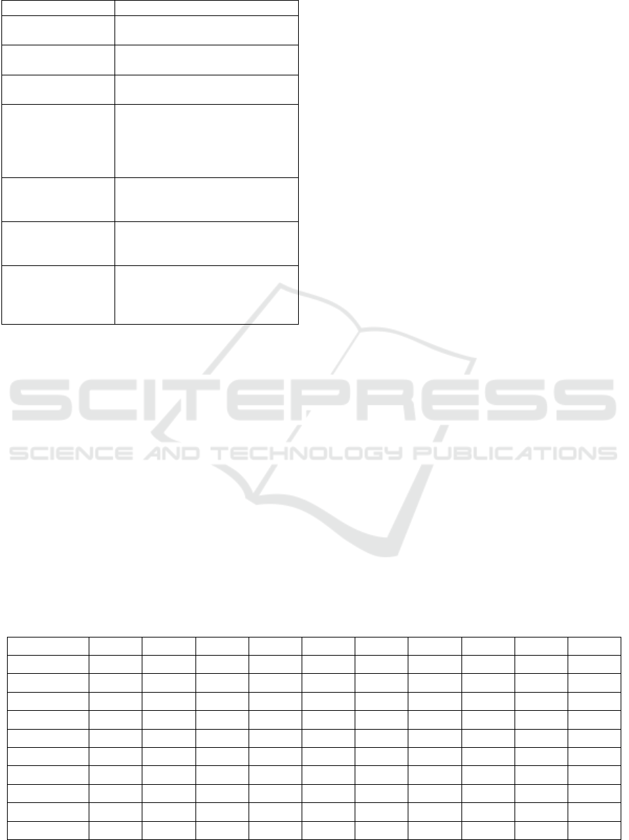
Table 1: Structural metrics for FM maintainability
assessing (Bagheri and Gasevic, 2011).
Metric Description
Number of features
(NF)
The total number of features that
are present in a feature model.
Number of leaf
features (NLeaf)
Number of the feature model tree
leaves.
Cyclomatic
complexity (CC)
The number of a feature model
integrity constraints.
Cross-tree
Constraints (CTC)
The ratio of the number of unique
features involved in the feature
model integrity constraint over all
of the number of features in the
feature model.
Ratio of variability
(RoV)
The average number of children
of the nodes in the feature model
tree.
Coefficient of
connectivity-
density (CoC)
The ratio of the number of edges
over the number of features in the
feature model.
Flexibility of
configuration (FoC)
The ratio of the number of
optional features over all of the
available features in the feature
model.
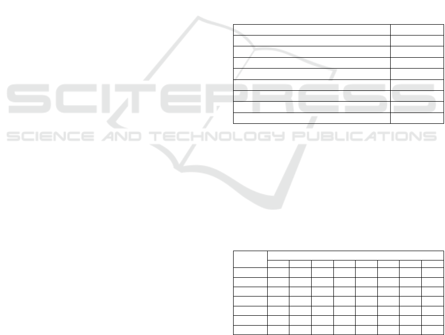
According to Bagheri and Gasevic, FM
maintainability is defined by three
subcharacteristics, which are analyzability,
changeability and understandability. “Analyzability
(An) is the capability of the conceptual model of a
software system to be diagnosed for deficiency;
changeability (Ch) is the possibility and ease of
change in a model when modifications are
necessary, and Understandability (Un) is the
prospect and likelihood of the software system
model to be understood and comprehended by its
users or other model designers” (Bagheri and
Gasevic, 2011). In table 2, we present a correlation
matrix realized by the mentioned authors. Table 2, is
a merge of three tables presented in (Bagheri and
Gasevic, 2011). It can be seen from table 2 that the
number of leaves (NLeaf) in a feature model has a
high negative correlation with both analyzability and
understandability (-0.86 and -0.82, respectively). In
turn, the number of features (NF) is also closely
correlated with these two characteristics (-0.75 and -
0.81). The correlation between NLeaf and NF and
these two sub characteristics of maintainability is
highly negative, then it can be deduced that more
features and leaf features a FM has more complex it
becomes in terms of analyzability and understand-
ability. Consequently, maintainability is worse.
3 PL EVOLUTION BY RL
In this section, we present the Reinforcement
Learning approach, and then we present our
motivations to introduce this approach in improving
FM maintainability.
3.1 Learning by Reinforcement
Reinforcement Learning is a subfield of Machine
Learning. One of its purposes is automatic decision-
making. In RL, an agent interacts with its
environment by perceiving its state and selecting an
appropriate action, either from a learned policy (by
experience) or by random exploration of possible
actions. As a result, the agent receives feedback in
terms of rewards, which rate the performance of its
previous action. In fact, an action is chosen by RL
using two complementary strategies: exploitation
and exploration. Exploitation focuses on the collected
reward values, and recommends the action with the
highest reward to be executed. Exploration
recommends a random action regardless of its reward
value to prevent the learning from sub-optimal
solutions. A proper learning strategy is a reasonable
combination of exploitation and exploration.
Table 2: Correlation matrix of FM maintainability parameters (Bagheri and Gasevic, 2011).
NF NLeaf CC CTC RoV CoC FoC An Un Ch
NF 1 0.95 0.41 0 -0.01 0.24 -0.53 -0.75 -0.81 -0.46
NLeaf 1 0.54 0.17 0.22 0.39 -0.59 -0.86 -0.82 -0.60
CC 1 0.8 0.65 0.91 -0.67 -0.48 -0.53 -0.92
CTC 1 0.78 0.93 -0.65 -0.21 -0.25 -0.80
RoV 1 0.69 -0.47 -0.39 -0.12 -0.63
CoC 1 -0.74 -0.36 -0.46 -0.89
FoC 1 0.49 0.74 0.73
An 1 0.74 0.60
Un 1 0.63
Ch 1
A Reinforcement Learning Approach to Feature Model Maintainability Improvement
391
3.2 Decision Making for Core Assets
Evolution
SPLs core assets include variabilities, constraints
and so many concepts to represent a family of
products. Evolving a core asset requires various
change operations. Many scenarios may occur, as
well. Making a decision for choosing the convenient
scenarios and operations to evolve a core asset is a
hard task. According to some experience reports
(O’Brien, 2001), (Bergey et al., 2010), some
decisions may lead to negative results. For example,
in (Bergey et al., 2010), the authors regret updating
some components in order to increase the flexibility
of their PL architecture. They spent seven months
for the updates but finally they rejected the new
components. Therefore, the decision to update an
asset instead of replacing it was not a good
recommendation. A decision maker as an automatic
process can be the solution to help human to choose
the best scenarios (sequence of operations) to evolve
their product lines. Particularly, a decision maker
proposed by a reinforcement learning approach can
optimize the improvements of FM maintainability. It
makes the decisions to pick the convenient evolution
(change) operations (e.g., add a feature and remove a
feature) on a FM to improve its maintainability.
4 FM MAINTAINABILITY
IMPROVEMENT BASED ON RL
Our proposal consists in the design of a RL-based
evolution agent. Its role is to help evolving PL
feature models by proposing the convenient change
operations to improve their maintainability. The
agent consists of three key components: quality
attribute monitor, decision maker, and evolution
controller. Hence, the role of the agent we propose is
to pick automatically the best evolution operations
for improving FM maintainability. Therefore, the
maintainability monitor measures the metrics related
to maintainability quality attribute (e.g., FoC, CC,
CTC, RoV, NLeaf and the CoC) (described in table
1). Then it sends the information to RL-based
decision maker. The decision maker runs the Q-
learning RL algorithm (Sutton and Barto, 2011) and
produces a state-action table, called Q-value table. A
state is defined by a version of a FM, which is
represented by a set of selected parameters (see table
3). Possible actions to change the state of a FM are
evolution (change) operations. They include adding
a leaf optional feature, removing a feature, changing
the optionality of a feature, adding a constraint,
removing a constraint, etc. Each action may act on
one or more parameters of the FM state. Based on
the dynamically updated Q table, the evolution
controller generates the evolution policy and evolves
the FM by creating a new version (state).
4.1 Parameters as FM Vector State
Dimensions
To represent a FM state we identified a set of
parameters, which are presented in table 3 and that
we can consider as a vector with 8 dimensions. In
table 4, we show which parameters are used by each
metric. For instance, in the running example (see
Figure 1), the values of these parameters are NLF=
12, TNF=17, TNE=16, TNOF=1, NIC=4, NCF=16,
NN=5 and NFIC=5.
Table 3: State vector dimensions.
Meaning Dimension
Number of leaf features NLF
Total number of features in a FM TNF
Total number of Edges in a FM TNE
Total number of optional features TNOF
Number of integrity constraints (ICs) NIC
Number of children features NCF
Number of nodes (not leaf nodes) NN
Number of features included in ICs NFIC
The formula of each metric considering the
selected parameters is defined as follows (Bagheri
and Gasevic, 2011): CC = NIC, CoC = TNE/TNF,
FoC = TNOF/TNF, RoV = NCF/NN, NLeaf = NLF
and CTC = NFIC/TNF. For instance, according to
the running example the values of these metrics are:
CC=4, CoC=0.94, FoC=0.059, RoV=3.2, NLeaf=12
and CTC=0.294.
Table 4: Metrics and state dimensions dependency.
Metrics
State dimensions
NLF TNF TNE TNOF NIC NCF NN NFIC
CC
NF
CoC
FoC
RoV
NLeaf
CTC
4.2 Decision Making
In our approach, we define a state by a version of a
FM to evolve. For the selective group of n
parameters (dimensions), we represent a state S
i
by a
ENASE 2021 - 16th International Conference on Evaluation of Novel Approaches to Software Engineering
392
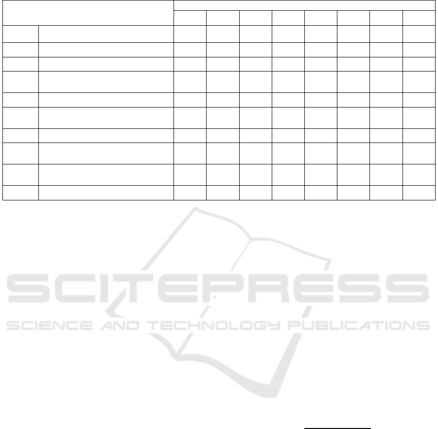
Table 5: Change actions and related dimensions.
Actions
Dimensions
NLF TNF TNE TNOF NIC NCF NN NFIC
A
0
Add-leaf-optional-feature
A
1
Add-leaf-mandatory-feature
A
2
Remove-leaf-optional-feature
A
3
Update-optionality-of-a-feature
(from Mandatory to Optional)
A
4
Add-constraint-on-two-features
A
5
Add-node-mandatory-feature with
two children leaf-optional
A
6
Remove-leaf-mandatory-feature
A
7
Update-optionality-of-a-feature
(from Optional to Mandatory)
A
8
Remove-node-mandatory-feature
with its two children leaf-optional
A
9
Remove a constraint on two features
vector in the following form: S
i
= (Para
1
, Para
2
, …,
Para
n
). To evolve the maintainability of a FM, a state
of a FM is represented by the vector: S
i
= (NLF,
TNF, TNE, TNOF, NIC, NCF, NN, NFIC). For
instance, the first (initial) version of the FM of the
running example is defined by the State S
0
= (12, 17,
16, 1, 4, 16, 5, 5).
We use a vector A
i
to represent an action on the
parameters (state dimensions) it affects. Each action
is a 8-elements vector, indicating influenced/not-
influenced (1/0) of the eight parameters. The action
vector is in the following form : A
i
=(1,1,1,0,0,0,0,0).
This means that action A
i
influences the first
parameter (NLF), the second parameter (TNF) and
the third parameter (TNE) of a FM state. However,
the next parameters are not impacted by the action
A
i
. For instance, the following notation represents
the influence of the action Add-leaf-optional-feature
(A
1
) on parameters NLF, TNF, TNOF and NCF :
A
1
(1,1,0,1,0,1,0,0).
The agent receives a reward value as the
feedback following the application of an action. For
our approach, the reward should reflect the FM
maintainability improvement. For a given action A
i
,
a set of parameters are affected. Consequently, the
values of the metrics based on these parameters are
impacted. Finally, the maintainability is influenced.
If the FM maintainability is improved then the agent
receives a positive reward else, it receives a negative
one. The overall aim of RL is to maximize some
form of cumulative reward. For instance, applying
the action A
1,
Add-leaf-optional-feature, influences
the values of the parameters NLF, TNF, TNOF and
NCF. Therefore, the values of the metrics NF,
NLeaf, CoC, FoC, CTC and RoV (see table 4) are
affected and finally the FM maintainability is
impacted. For our approach, we are based on the
affected metrics and their correlation coefficients
with the subcharacteristics of maintainability as
indicators to deduce the reward value.
First, we pick the metrics related to the parameters
affected by the applied action (see table 5). Then, the
reward value r
t
is defined at instant t (when the
action is applied) based on the value of the
standardized Cronbach’s alpha (coefficient alpha)
(NCSS, 2021). Coefficient alpha is the most popular
of the internal consistency coefficients. We use the
standardized expression of Cronbach’s alpha
because its calculation is based on a correlation
matrix (see equation 1).
𝛼=
𝑘𝜌
̅
1+ 𝜌
̅
(𝑘 − 1)
(1)
The parameter k is the number of items (variables)
and ρ is the average of all the correlations among k
items.
The reward value at instant t may be 1, 0 or -1.
Alpha (α) is calculated for the sub-matrix extracted
from the correlation matrix of table 2. This sub-
matrix contains the correlation coefficients of the
picked metrics (impacted by action taken at instant t)
and the maintainability sub characteristics. Then the
average of the new values of the metrics is
calculated (AV
new
). We consider as AV
old
the
average of these metrics before applying the action
of instant t. The reward value R (or r
t
) is defined as
A Reinforcement Learning Approach to Feature Model Maintainability Improvement
393

follows: a) if α is high negative and AV
new
> AV
old
then R = -1 because maintainability is worse. b) If α
is high positive and AV
new
> AV
old
then R = 1
because maintainability is better. c) If α is high
positive and AV
new
< AV
old
then R= -1 because
maintainability is worse. d) If α is high negative and
AV
new
< AV
old
then R = 1 because maintainability is
better. e) If AV
new
= AV
old
then R = 0 because
maintainability is not impacted.
To learn the Q value of each state, the agent
should continuously update its estimation based on
the state transition and reward it receives. Using
such incremental fashion, the average Q value of an
action A on state S, denoted by Q(S, A), can be
refined once after each reward R is collected (see the
equation 2).
𝑄
(
𝑆, 𝐴
)
=𝑄
(
𝑆, 𝐴
)
+𝛼
𝑅+𝛾 𝑚𝑎𝑥
𝑄
(
𝑆
,𝑎
)
−𝑄
(
𝑆, 𝐴
)
(2)
The parameter α is the learning rate; its value is
between 0 and 1. We note that alpha used in this
expression is not the standardized Cronbach’s alpha
(no relationship between them). The parameter γ is
the discount factor; it is set between 0 and 1. max
a
Q(S’, a) indicates the maximum reward that is
attainable in the state following the current one; i.e.,
the reward for taking the optimal action thereafter.
A
lgorithm 1: Q-value Learning Algorithm.
1 : Initialize Q-table
2 : Initialize state S
3 : Repeat (for each state)
4 : Choose action A for state S using ε-
greedy policy
5 : Take action A, observe R and S’
6 :
Q(S, A) = Q(S, A) + α[R
+
γ
max
a
Q(S’, a) - Q(S, A)]
7 :
S
← S’
8 : Until terminal state
Algorithm 1 presents the pseudo code of our Q-
value learning algorithm. It is explained as follows:
1) Initialize the Q-values table, Q(S, A). 2) Initialize
the first state of the FM, 3) Observe the current state
S. 4) Choose an action, A, for that state based on the
policy ε-greedy (Sutton and Barto, 2011). The agent
then picks the action based on the max value of
those actions. This is exploiting since decision is
made from available information. The second way to
take action is to act randomly. This is exploring.
Instead of selecting actions based on the max future
reward, an action is selected at random. We can
balance exploration/exploitation using epsilon (ε)
and setting the value of how often you want to
explore vs exploit. 5) Take the action, and observe
the reward, R, as well as the new state, S’. 6) Update
the Q-value for the state using the observed reward
and the maximum reward possible for the next state.
The updating is done according to the formula and
parameters described above. 7) Set the state to the
new state, S’, and repeat the process until 8) a
terminal state is reached. In our work, we consider a
terminal state as a FM version fixed by the domain
(product line) expert.
5 APPROACH EXPERIMENT
In this section, we present an application of the
approach we propose to the GPL feature model
(shown in figure 1). We implemented the approach
with Python. Following, we present the algorithm 1
application.
The Q-table is defined by 10 actions (see table 5)
and 8 states of the FM. The state number 7
represents the terminal FM version to be reached. In
Q-table initialization, we set all the values of the
state-action pairs to zero since all the actions for
each state are assumed to be an equally valid choice.
This approach starts the system from an initial state
of a FM. Then actions are applied according to the
algorithm 1. In our case, the running example (see
figure 1) is the initial FM. Its state is represented by
the vector S
0
= (12, 17, 16, 1, 4, 16, 5, 5) as defined
above.
We wanted that exploration is higher than
exploitation because the agent has to learn more than
to exploit applied actions. Consequently, we chose a
value of epsilon = 0.9. We set the learning rate α =
0.1 in order to make the agent explores more states
and γ=0.9 to consider the future rewards as
important. Table 6 shows the Q-table after 800
iterations of Q-learning. Each Q-value (Si, Ai)
corresponds to the probability to improve the FM
state Si by applying the action Ai. For each state, we
underline the maximum Q-value in order to show
the maximum probability to indicate the best action
to improve that state. For instance, in the line of
state S0, the maximum value is 0.86 and its
corresponding action is A6. This means that
choosing the action A6 has the probability of 0.86 to
improve the state S0 of the FM maintainability. We
can observe in table 6 that actions 2 and 7 are never
taken (their Q-values are null). Then more
exploration is needed. Table 7 shows the Q-table
following the decrease of the learning rate α to 0.02
ENASE 2021 - 16th International Conference on Evaluation of Novel Approaches to Software Engineering
394
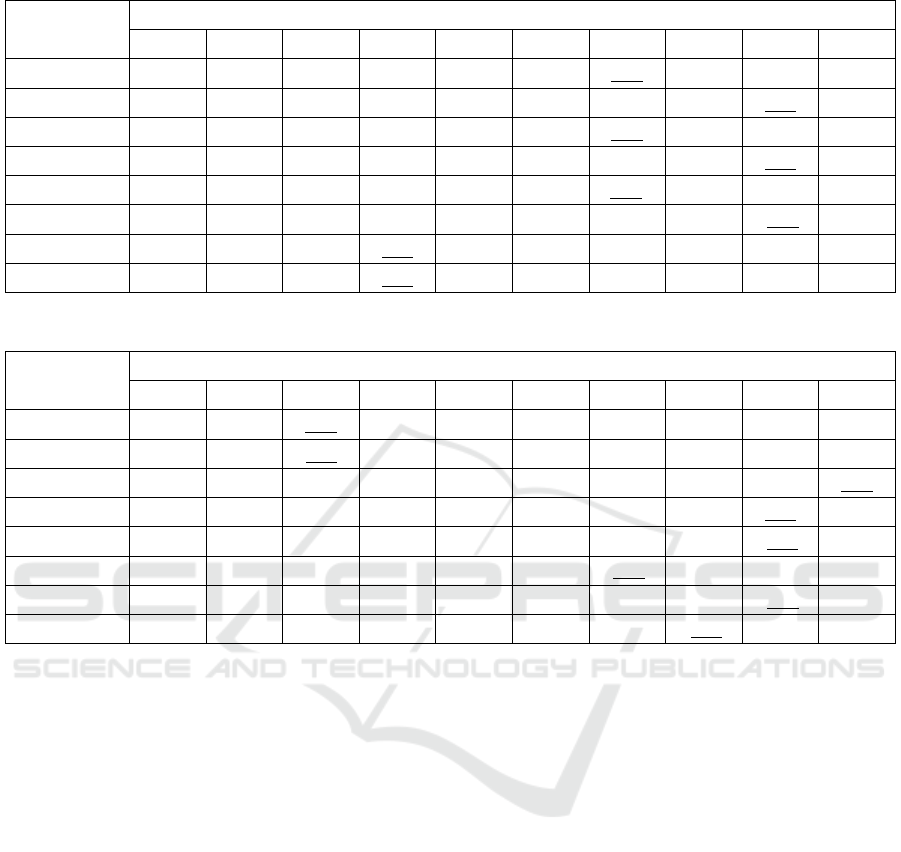
Table 6: Q-Table values after 800 iterations of learning (α = 0.1, γ=0.9 and ε=0.9).
States
Actions
A0 A1 A2 A3 A4 A5 A6 A7 A8 A9
S0 0.5 0.4 0 0.05 0.8 0.1 0.86 0 0.85 0.08
S1
0.17 0.75 0 0.07 0.39 0.04 0.07 0 0.98
0.04
S2
0.15 0.35 0 0.01 0.09 0.03 0.53
0 0.2 0.06
S3
0.15 0.16 0 0.1 0.71 0.01 0.04 0 0.73
0.23
S4
0.12 0.72 0 0.05 0.41 0.01 0.83
0 0.80 0.33
S5
0.31 0.84 0 0.02 0.74 0.04 0.06 0 0.92
0.48
S6
0.41 0.09 0 0.52
0.45 0.08 0.41 0 0.33 0.50
S7
0.51 0.52 0 0.72
0.07 0.07 0.06 0 0.69 0.07
Table 7: Q-Table values after 800 iterations of learning (α = 0.02, γ=0.9 and ε=0.9).
States
Actions
A0 A1 A2 A3 A4 A5 A6 A7 A8 A9
S0 0.42 0.32 0.75 0.01 0.6 0.11 0.35 0.52 0.36 0.45
S1
0.18 0.54 0.68
0.15 0.59 0.04 0.07 0.56 0.58 0.67
S2
0.54 0.35 0.35 0.01 0.02 0.03 0.03 0.65 0.33 0.85
S3
0.35 0.16 0.12 0.1 0.11 0.01 0.47 0.15 0.73
0.09
S4
0.34 0.26 0.15 0.05 0.41 0.01 0.03 0.25 0.87
0.12
S5
0.42 0.56 0.13 0.02 0.74 0.04 0.92
0.29 0.91 0.87
S6
0.52 0.33 0.25 0.02 0.66 0.08 0.1 0.86 0.88
0.45
S7
0.3 0.51 0.26 0.45 0.07 0.07 0.06 0.87
0.69 0.36
in order to increase the learning by exploring more
states.
We noted that Actions 2 and 7 are taken
(explored). In addition, we observed that the Action
2 has the probability of 0.75 to improve the
maintainability of the FM in state S
0
. This indicates
that more learning may lead to new decisions.
6 RELATED WORK
Many past works were devoted to feature models
evolution. In this section, we present approaches
related to our proposal. In (Bhushan et al., 2018), the
authors proposed an ontology-based approach for
identifying inconsistencies in FMs, explaining their
causes and suggesting corrective solutions. The
ontology is used to express the semantic of feature
models. Rules in FOL (first order logic) are defined
to express constraints on FMs consistency. This
approach is about improving the quality of FMs,
where the quality attribute is consistency. However,
learning is not considered in this work as in our
approach where we also treat several quality
attributes.
In order to improve usability of FMs, Geetika
and al. (Geetika et al., 2019) proposed a prediction
approach to estimate FMs usability. Five machine
learning algorithms were used to compare their
prediction accuracy in terms of usability to predict
FMs usability. The authors used a set of metrics to
express FMs information and sub-characteristics to
express the usability quality attribute related to FMs.
This work is not validated and there is no result.
To evolve FMs automatically, in (Ren et al.,
2019), the authors proposed a method of
automatically generating the evolved SPL’s feature
models. The evolution process takes an initial FM
and evolutionary requirements as input and produces
an evolved FM. Their approach uses a formal
method named communication membrane calculus
to describe the structure of feature models and
evolution process of feature models. This approach
is about FM evolution but it is not based on learning.
Other proposed works, which are related to our
approach are dedicated to dynamic SPLs such as in
A Reinforcement Learning Approach to Feature Model Maintainability Improvement
395

(Pessoa et al., 2017) where an approach was
proposed to build reliable and maintainable DSPLs.
Adaptation plans are used at runtime. The proposed
approach was applied and evaluated on the body
sensor network domain. The results showed that
reliability and maintainability are provided with
execution and reconfiguration times. Hence, their
work is interested in quality attributes of DSPLs but
no learning is done. In (Xiangping et al., 2009) a
reinforcement approach is proposed to auto-
configure online web systems. In DSPL, context
change leads to change in system configuration.
Then, the authors used Q-learning reinforcement
learning to detect change in the workload and the
virtual machine resource of the online web system
and to adapt the system configuration (performance
parameter settings). Where this work uses the Q-
learning algorithm as in our approach, its goal is to
automate configurations of DSPL online web
systems. According to existing works, our
contribution, which is RL-based, seems promising,
considering different FM quality attributes to
maintain where change operations occur on FM.
7 CONCLUSION
Product Line evolution is a continuous process
where the improvement of PLs core assets quality
attributes is mandatory. What are the elements that
we may change and when their change is reasonable
are hard decisions. Learning by experience to make
a decision is a good approach. Consequently, using
an automatic decision maker to help PL
organizations to do the right changes in their core
assets is a challenge. In order to tackle this latter, we
proposed a reinforcement learning approach to FM
evolution. Our approach makes decisions about
change operations on feature models to improve
their maintainability. However, further
experimentations are required to validate our results
and draw last conclusions. In fact, we can extract
more FMs from SPLOT repository to apply the
proposed approach and to give better interpretations.
In our approach we use structural metrics to
assess the FM maintainability and then to obtain the
reward value. These metrics are not sufficient
because some change operations on the FM do not
affect them. Therefore, the impact of these
operations on the FM maintainability is not
considered. Examples of these change operations are
change the dependency of a node with its children
from OR to AND, change the name of a feature, add
a feature cardinality and add group cardinality.
Consequently, the other directions of future work
that we are interested in are: 1) exploring and
studying metrics related to the FM semantic, 2)
defining our correlation matrix considering various
types of metrics to determine FM maintainability.
REFERENCES
Clements, P., Northrop, L., 2001. Software Product Lines:
Practices and Patterns, Addison-Wesley Professional.
Lopez-Herrejon, R. E., Batory, D., 2001. A standard
problem for evaluating product-line methodologies.
In: Bosch J. (eds) Generative and Component-Based
Software Engineering. GCSE 2001. Lecture Notes in
Computer Science, vol 2186. Springer, Berlin,
Heidelberg.
NCSS statistical software, 2021. Correlation Matrix.
NCSS, LLC. All Rights Reserved, (NCSS.com).
Bagheri, E., Gasevic, D., 2011. Assessing the
maintainability of software product line feature models
using structural metrics. Software Quality J, pp. 579–
612.
O’Brien, L., 2001. Architecture Reconstruction to Support
a Product Line Effort: Case Study, Technical Note
CMU/SEI-TN-015.
Bergey, J. K., Chastek, G., Sholom, C., Donohoe, P.,
Jones L. G., Northrop, L., 2010. Software Product
Lines: Report of the U.S. Army Software Product Line
Workshop, Technical Report, Software Engineering
Institute, CMU/SEI Report Number: CMU/SEI-2010-
TR-014.
Xiangping, B., Jia, R., Cheng-Zhong, X., 2009. A
Reinforcement Learning Approach to Online Web
System Auto-configuration, ICDCS '09: Proceedings
of the 29th IEEE International Conference on
Distributed Computing SystemsJune pp. 2–11.
Bhushan, M., Goel, S., Kumar, A., 2018. Improving
quality of software product line by analysing
inconsistencies in feature models using an ontological
rule-based approach, Expert Syst. J. Knowl. Eng.
Pessoa, L., Fernandes, P., Castro, T., Alves, V.,
Rodrigues, G.N., Carvalho, H., 2017. Building reliable
and maintainable dynamic software product lines: an
investigation in the body sensor network domain, Inf.
Softw. Technol. 86 pp54–70.
Geetika, V., Sonali, V., Prasanta, K. P., Amita, S., Chitra,
B., 2019. Prediction Algorithms and Consecutive
Estimation of Software Product Line Feature Model
Usability, Computer Science, Amity International
Conference on Artificial Intelligence (AICAI).
Ren, J., Liu, L., Zhang, P., Wenbo, Z., 2019. A Method of
Automatically Evolving Feature Models of Software
Product Lines, Computer Science, IEEE.
Sutton, R. S., Barto, A., G., 2011. Reinforcement
Learning: An Introduction (Adaptive Computation and
Machine Learning Series), Kindle Editions, ISBN
978-o-262-30384-2 (e-book).
ENASE 2021 - 16th International Conference on Evaluation of Novel Approaches to Software Engineering
396
