
Entropy Map Might Be Chaotic
Junping Hong
a
and Wai Kin (Victor) Chan
b
Tsinghua-Berkeley Shenzhen Institute, Tsinghua University, Shenzhen, China
Keywords: Chaos, Chaotic Map, Information Entropy, Julia Set, Frobenius-Perron Operator.
Abstract: Chaos is a phenomenon observable in many areas. Chaotic behaviours can be visualized in chaotic maps, which
are deterministic iterative functions and sensitive to initial conditions. As a result, they are wildly adopted in
random number generator, image encryption, etc. In this paper, two new chaotic maps inspired by information
entropy are proposed. Through bifurcation diagram and Lyapunov exponent analysis, period doubling
bifurcations are observed and chaos is suggested. Furthermore, these maps lead to a special case of the Frobenius-
Perron operator in their distributions and are extended to the complex plane to obtain the Julia set.
1 INTRODUCTION
Chaos is a nonlinear phenomenon in the physical
world. First proposed by Lorenz (Lorenz, 1963), a
chaotic system is a deterministic system sensitive to
initial conditions: a small change at the beginning can
magnify into large variations in the long term.
Chaotic maps are iterative functions in dynamics
systems that exhibit chaotic behaviour for special
parameters of the related function. They can be
classified as discrete or continuous for real or
complex variables. The Lorenz system, for instance,
is a continuous chaotic map.
One-dimensional chaotic maps are discrete
chaotic maps. They became popular research areas
since the discovery of the Logistic Map in 1976. May
discovered that these simple mathematical models
could lead to complicated dynamics (May, 1976).
Afterwards, more chaotic maps had been found,
including classical maps like Tent Map (Devaney,
1984), Sine Map (Strogatz, 1994), and Doubling Map
(Hirsch et al., 2013). Chaotic maps are useful in
random number generator and image encryption due
to their deterministic properties and high sensitivities
to initial conditions.
In recent years, numerous additional chaotic maps
have been proposed and analysed. Alpar constructed
a simple fraction in a square map with one variable
and two parameters, and studied this map through
stability bifurcation, Lyapunov exponents, and
a
https://orcid.org/0000-0002-3341-7406
b
https://orcid.org/0000-0002-7202-1922
cobweb plot analysis (Alpar, 2014). A novel one-
dimensional sine powered chaotic map was proposed
and applied in a new image encryption scheme by
Mansouri et al. (2020). Lambić proposed a new
discrete chaotic map according to the composition of
permutations (Lambić, 2015).
When discrete chaotic maps involve complex
variables, they can be represented as Julia sets. In
general, a Julia set is a fractal in the complex plane
(Peitgen et al., 2004) defined as the following
(Falconer, 2014): First, take 𝑓: C → C as mapping
function with complex parameter. Usually, 𝑓
is the
k composition 𝑓∘⋯∘𝑓, and 𝑓
𝜔 is the k-th
iteration 𝑓𝑓⋯𝑓𝜔⋯. Then, the filled-in Julia
set becomes:
𝐾
𝑓
=
𝑧∈𝐶:
𝑓
𝑧 ↛ ∞
(1
)
The Julia set of 𝑓 is the boundary of filled-in Julia
set, 𝐽𝑓 𝜕𝐾𝑓. If every neighbourhood of 𝑧 exists
different points of 𝜔 and 𝜐, such that 𝑓
𝜔 →∞, and
𝑓
𝜐 ↛∞, then 𝑧 belongs to the Julia set 𝐽𝑓.
Julia sets have a number of applications in the arts,
computer science, and finance. For example, Cui et
al. extended the Black-Scholes model to find the
fractal in the model, which was a function for pricing
European option (Cui et al., 2016).
In this research, we propose two new iterative
functions based on the information entropy formula.
The main goal of this paper is to show that they are
86
Hong, J. and Chan, W.
Entropy Map Might Be Chaotic.
DOI: 10.5220/0010469700860090
In Proceedings of the 6th International Conference on Complexity, Future Information Systems and Risk (COMPLEXIS 2021), pages 86-90
ISBN: 978-989-758-505-0
Copyright
c
2021 by SCITEPRESS – Science and Technology Publications, Lda. All rights reserved
chaotic through bifurcation diagram and Lyapunov
exponent analysis. The rest of the paper is organized
as follows. The new chaotic maps are proposed in
Section 2. In Section 3, we verify these two maps are
chaotic through bifurcation diagram and Lyapunov
exponent. Their distributions are also analysed due to
the emergence of an interesting phenomenon. In
Section 4, we extend the new chaotic maps to
complex plane to obtain the Julia sets. Finally,
Section 5 concludes the paper with discussions.
2 NEW ONE-DIMENSION
CHAOTIC MAPS
Information Entropy was introduced by Shannon in
his famous paper “A Mathematic Theory of
Communication”, where he estimated the uncertainty
of random variable (Shannon, 1948):
𝐻 = 𝐾
∑
𝑝
𝑙𝑜𝑔𝑝
(2)
where H denote information entropy, and K is a
positive constant.
Based on the above information entropy formula,
we propose two new iterative functions (eq.3 and
eq.4):
𝑥
= 𝛼𝑥
𝑙𝑛𝑥
(3)
where n is the iteration number, 𝛼 the control
parameter, 𝑥
∈0,1, and 𝛼∈0,𝑒. And
𝑥
= 𝛼𝑥
𝑙𝑛𝑥
𝑥
𝑙𝑛𝑥
(4)
where, 𝑥
denotes (1𝑥
), 𝛼 the control parameter,
𝑥
∈ 0,1, and 𝛼∈0,
.
3 ANALYSIS
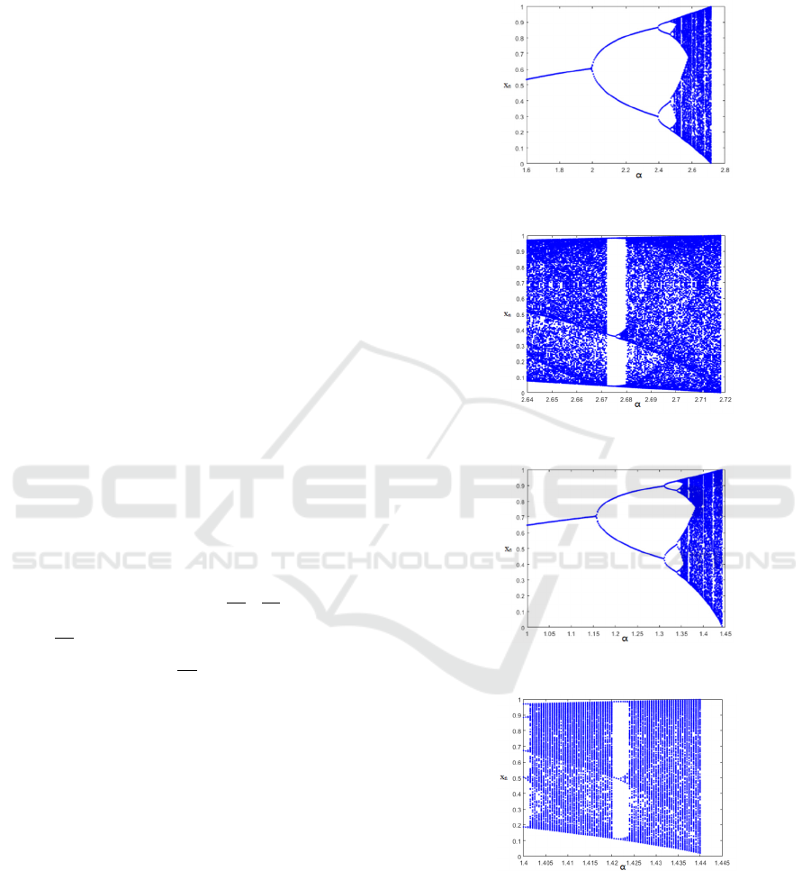
3.1 Bifurcation Diagram
Bifurcation diagram is used to analyse the behaviour
of chaotic map, which plots possible long-term values
of the dynamic system as a function of one of its
parameters. Normally, there are period doubling
bifurcation and “period of 3”. Observance of the
“period of 3” in the bifurcation diagram implies chaos
(Li et al., 1975).
The bifurcation diagrams of eq.3 and eq.4 are
given in fig.1-2 and fig.3-4, respectively. There are
clear period doubling bifurcation and chaotic region
on the right size with a few numbers of periodic
windows on the left. In the bifurcation diagrams fig.2
and fig.4, the window of “period of 3” can be clearly
observed.
Figure 1: Bifurcation diagram of eq.3.
Figure 2: “Period of 3” of eq.3.
Figure 3: Bifurcation diagram of eq.4.
Figure 4: “Period of 3” of eq.4.
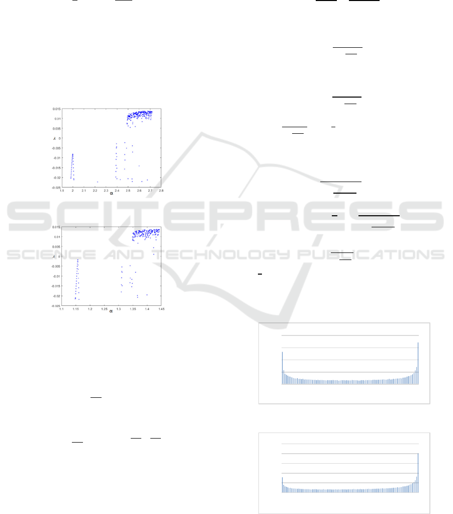
3.2 Lyapunov Exponent
The Lyapunov exponent 𝜆 is a strong instrument to
measure a system’s sensitivity to slight changes in the
initial condition. 𝜆 quantifies the average increment
of an infinitely small error at the initial point. 𝜆0
Entropy Map Might Be Chaotic
87
indicates that the dynamic system is sensitive to the
initial condition; 𝜆0 means the system is stable;
and 𝜆0 reflects that the system tends to stabilize.
If the 𝜆 for a one-dimensional chaotic map is positive,
chaos is implied (Hao, 1993).
According to Peitgen et al. (2004), 𝜆 can be
calculated as follows:
𝜆 =
∑
𝑙𝑛|
|
(5
)
where n is the iteration number and 𝐸
the error in the
k-th iteration.
Fig.5 and fig.6 show that the largest 𝜆 of these two
maps are around 0.014, which is relatively small.
Results suggest that the chaotic maps of information
entropy are less chaotic compared to other chaotic
maps.
Figure 5: Lyapunov exponent of eq.3.
Figure 6: Lyapunov exponent of eq.4.
3.3 Distribution
Previous results indicate that eq.3 and eq.4 have
chaotic regions. In the chaotic region, let parameter 𝛼
equal to 𝑒 in eq.6 and
in eq.7.
𝑥
= 𝑒𝑥
𝑙𝑛𝑥
(6)
𝑥
=
𝑥
𝑙𝑛𝑥
𝑥
𝑙𝑛𝑥
(7)
Fig.9 and fig.10 show the approximate
distributions for eq.6 and eq.7. One interesting
phenomenon is that the distribution of eq.7 is not
symmetric while the function has an axis of symmetry
around 𝑥0.5.
Here we show that the probability density
function of eq.7 would not be symmetric if it is
monotone in [0, 0.5]. Let y denote 𝑋
and x denote
𝑋
. Let 𝜐𝑦 denote the probability density function
of y and 𝜐𝑥 denote the probability density function
of x. Based on the Frobenius-Perron function (Peitgen
et al., 2004):
𝜐𝑦 =
||
||
(8
)
Assume that 𝜐𝑥 𝜐1 𝑥, then:
𝜐𝑦 =
|
|
(9
)
Integrate from 0 to 1:
𝜐𝑦𝑑𝑦
|
|
𝑑𝑥
=1
(10
)
|
|
𝑑𝑥
.
=
(11
)
Using Chebyshev integral inequalities:
𝜐𝑥
.
𝑑𝑥
𝑙𝑛2
|ln
1𝑥
𝑥
|
.
𝑑𝑥
1
2
𝜐𝑥𝑙𝑛2
|ln
1𝑥
𝑥
|
𝑑𝑥
.
(12
)
We show that
|
|
.
𝑑𝑥 should be no larger
than
while simple calculation shows it is. There is
clearly a contradiction. So the probability density
function would not be symmetric if it is monotone in
[0, 0.5].
Figure 7: Distribution of eq.6.
Figure 8: Distribution of eq.7.
0
0,02
0,04
0,06
0,08
0,01
0,07
0,13
0,19
0,25
0,31
0,37
0,43
0,49
0,55
0,61
0,67
0,73
0,79
0,85
0,91
0,97
0
0,02
0,04
0,06
0,08
0,1
0,01
0,07
0,13
0,19
0,25
0,31
0,37
0,43
0,49
0,55
0,61
0,67
0,73
0,79
0,85
0,91
0,97
COMPLEXIS 2021 - 6th International Conference on Complexity, Future Information Systems and Risk
88
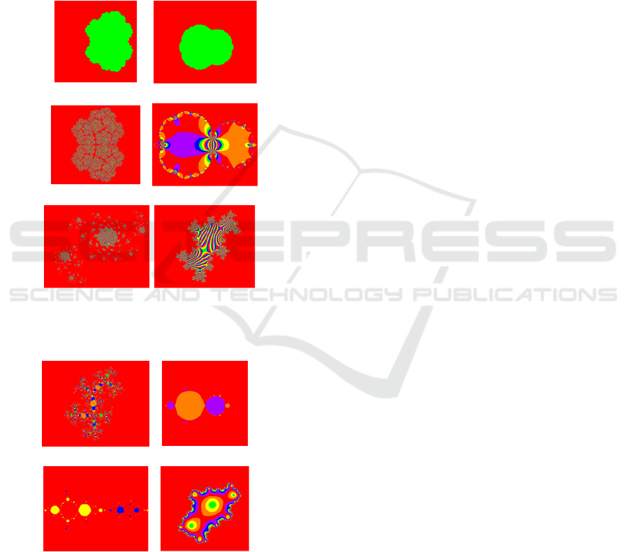
4 JULIA SET
In this part, we calculate for the Julia set by
constructing two iterative functions (eq.13 and eq.14)
on the complex plane.
𝑧
= 𝑧
ln𝑧
c
(13)
𝑧
= 𝑧
lnz
c
(14)
Fig.9 and fig.10 display the Julia sets for eq.12
and eq.13 with different values of c, respectively.
(a) (b)
(c) (d)
(e) (f)
Figure 9: Julia set of eq.13. (a) c = 0; (b) c=0.75; (c) c = -
0.15; (d) c=1; (e) c = 0.8+0.6i; (f) c=0.7i.
(a) (b)
(c) (d)
Figure 10: Julia set of eq.14. (a) c = -0.42i; (b) c=3; (c) c =
4; (d) c=2+1i.
5 CONCLUSIONS AND
DISCUSSION
In this study, we propose two new chaotic maps,
which are inspired by information entropy. Test and
analysis results suggest that they are chaotic, with
relatively small positive Lyapunov exponents around
0.014. In addition, we extend the chaotic maps to the
complex plane and obtain the Julia sets.
In the distribution of eq.7, asymmetry seems to
arise from a symmetry map. This might be caused by
the computational software, or the map itself. This
special Frobenius-Perron question remains unknown.
Future work can attempt to calculate the exact
distribution to answer this question and apply these
chaotic maps and Julia sets to new applications in
image encryption, finance, random number
generation and other applications.
REFERENCES
Alpar, O. (2014). Analysis of a new simple one dimensional
chaotic map. Nonlinear Dyn 78, pages 771–778.
Cui, Y., Rollin, S.D.B, Germano, G. (2016). Stability of
calibration procedures: fractals in the Black-Scholes
model. arXiv preprint arXiv:1612.01951
Devaney, R.L. (1984). A piecewise linear model for the
zones of instability of an area-preserving map. Phys.
D 10(3), pages 387–393.
Falconer, K. (2003). Fractal Geometry. John Wiley &
Sons. 2
nd
edition.
Feigenbaum, M.J. (1978). Quantitative Universality for a
Class of Nonlinear Transformations. Journal of
Statistical Physics, Vol.19, No.1.
Hao, B. (1993). Starting with Parabolas—An Introduction
to Chaotic Dynamics. Shanghai scientific and
Technological Education Publishing House. Shanghai,
China.
Hirsch, M.W., Smale, S., Devaney, R.L. (2013).
Differential equations, dynamical systems, and an
introduction to chaos. Academic Press, Amsterdam, 3
rd
edition.
Lambić, D. (2015). A new discrete chaotic map based on
the composition of permutations. Chaos, Solitons &
Fractals, Volume 78, September 2015, Pages 245-248.
Li, T., Yorke, J.A. (1975). Period 3 implys chaos. The
American Mathematical Monthly, Vol. 82, No. 10,
pages 985-992.
Lorenz, E.N. (1963). Deterministic Nonperiod Flow. J
Atmos Sci, 20, pages 130–141
Mansouri, A., Wang, X. (2020). A novel one-dimensional
sine powered chaotic map and its application in a new
image encryption scheme. Information Sciences,
Volume 520, May 2020, pages 46-62.
May, R.M, (1976). Simple mathematical models with very
complicated dynamics. Nature 261, 459–465.
Entropy Map Might Be Chaotic
89

Peitgen, H.O., Jürgens, H., Saupe, D. (2004). Chaos and
Fractals. Springer-Verlag New York Inc. New York,
2
nd
edition.
Shannon, C.E. (1948). A Mathematical Theory of
Communication. The Bell System Technical Journal,
Vol. 27, pp. 379–423, 623–656.
Strogatz, S.H. (1994). Nonlinear Dynamics and Chaos with
Applications to Physics, Biology, Chemistry and
Engineering. Perseus Books, New York.
COMPLEXIS 2021 - 6th International Conference on Complexity, Future Information Systems and Risk
90
