
Analysis Layer Implementation Method for a Streaming Data
Processing System
Aleksey Burdakov
1a
, Uriy Grigorev
1b
, Andrey Ploutenko
2c
and Oleg Ermakov
1d
1
Bauman Moscow State Technical University, Moscow, Russia
2
Amur State University, Blagoveschensk, Russia
Keywords: Streaming Processing, Analysis Layer, Sketch, Count-Min Sketch Algorithm.
Abstract: Analysis is an important part of the widely used streaming data processing. The frequency of flow element
occurrence and their values sum are calculated during analysis. The algorithms like Count-Min Sketch and
others give a big error in restoring the aggregate with a large number of elements. The article proposes
application of a vector matrix. Each vector has a length of 'n'. If the number of different elements approaches
'n', then the window size is automatically reduced. This allows accurate storage of the aggregate without
element loss. The SELECT operator for searching in a vector array is also proposed. It allows getting various
slices of the aggregated data accumulated over the window. The comparison of the developed method with
the Count-Min Sketch data processing method in the Analysis Layer was performed. The experiment showed
that the method based on the vector matrix more than twice reduces memory consumption. It also ensures
the exact SELECT statement execution. An introduction of a floating window allows maintaining the
calculation accuracy and avoiding losing records from the stream. The same query sketch-based execution
error reaches 200%.
1 INTRODUCTION
High performance streaming processing is required
for many applications such as financial trackers,
intrusion detection systems, network monitoring,
sensor networks, and others (Basat et al., 2018; Yan
et al., 2018; Poppe et al., 2020; Zhang et al., 2018).
These applications require time and memory efficient
algorithms. This is necessary to cope with high-speed
data streams (Basat et al., 2018).
Source (Psaltis et al., 2017) proposes a holistic
approach to organizing data streaming. The
corresponding architectural diagram includes the
following layers:
- data collection,
- message queue,
- analysis,
- in-memory data storage,
- data access.
a
https://orcid.org/0000-0001-6128-9897
b
https://orcid.org/0000-0001-6421-3353
c
https://orcid.org/0000-0002-4080-8683
d
https://orcid.org/0000-0002-7157-4541
Below is a brief description of the data streaming
layers.
1. Data Collection Layer. The flow pattern is used
here. The data comes from mobile devices (or media).
They are preliminarily saved in logs in order to
increase the system reliability (logging using RBML,
SBML, HML methods). Then the data is transferred
to the next layer input.
2. Message Queue Layer. The messaging tool
examples are: NSQ, ZeroMQ, Apache Kafka. One of
the most popular solutions is the Apache Kafka
project. It differs from peers in its reliability and the
provision of exactly-once semantics (Narkhede et al.
2017). It allows publishing and subscribing to
message streams.
There are three main components in this layer:
producer (data collection layer), broker, consumer
(analysis layer). Figure 1 shows the message
exchange diagram.
262
Burdakov, A., Grigorev, U., Ploutenko, A. and Ermakov, O.
Analysis Layer Implementation Method for a Streaming Data Processing System.
DOI: 10.5220/0010465902620269
In Proceedings of the 6th International Conference on Internet of Things, Big Data and Security (IoTBDS 2021), pages 262-269
ISBN: 978-989-758-504-3
Copyright
c
2021 by SCITEPRESS – Science and Technology Publications, Lda. All rights reserved
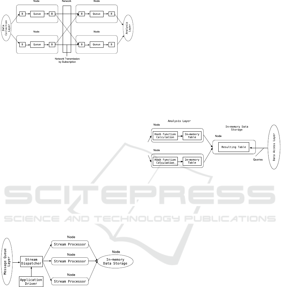
Figure 1: Broker Schema.
The broker component is designated with “B”.
Messages are received from the data collection layer.
The broker queues them up and then based on
subscription (“pushes”) them to the receiving broker.
It puts messages into the output queue. The analysis
layer sends requests to the broker and reads ("pulls")
messages from the queue.
Depending on the broker implementation, “push”
can be replaced with “pull” and vice versa. Brokers
are combined into a logical cluster. The message
queue layer parameters must be selected so that there
is no queue overflow. The work of brokers must be
simulated using a queuing system (Wu et al., 2019;
Kroß et al., 2016).
3. Analysis Layer. There is a number of data
analysis technologies. The most popular open source
products are Spark Streaming, Storm, Flink and
Samza (Quoc et al., 2017; Chintapalli et al., 2016;
Noghabi et al., 2017). They are all Apache projects.
The listed systems have a number of common
features (Psaltis, 2017) (Fig. 2).
Figure 2: Analysis Layer Schema.
Messages from the message queue layer are
bundled into packets. They accumulate in the system
over a certain time interval Δ. The streaming
dispatcher then distributes the packets to the stream
processors, which are processed by analysis
applications. It is important that the processing is
completed in less than Δ. The stream processor is
called differently: “Spark worker” in Spark
Streaming, “supervisor” in Storm, “worker” in Flink,
and “job worker Samza” in Samza. The analysis
applications can be different:
- counting unique values based on bit
combinations, for example, LogLog, HyperLogLog,
HyperLogLog
++
algorithms (Flajolet et al., 2017;
Heule et al., 2013), or based on ordinal statistics, e.g.
MinCount algorithm (Giroire, 2005),
- counting the frequency and sum of element
values in the stream, e.g. the Count-Min Sketch
algorithm (Cormode et al., 2005),
- determining whether the value was encountered
in the stream earlier (Bloom filter-based algorithm
(Bloom, 1970; Tarkoma et al., 2012)),
- other algorithms.
4. In-memory Data Storage. Hash functions are
calculated for the incoming elements, and the
resulting values are accumulated (or updated) in each
streaming process table (Fig. 3).
Figure 3: In-memory Data Store Schema.
The analysis applications listed in item 3 have the
property of linearity. The tables obtained in nodes can
be sent to one node and merged there. The union
consists in performing operations on the
corresponding cells of the source tables (counting
unique values, summing, etc.). The resulting table is
often referred to as a sketch (Chen et al., 2017). Hash
functions calculation, accumulating or updating
tables is quick. Each table size is a few KB, so their
network transfer is very quick.
5. Data Access Layer. There are many interaction
patterns between a streaming client (data receiver)
and a data warehouse (Psaltis, 2017): data
synchronization (Data Sync), remote method or
procedure calls (RMI / RPC), simple messaging,
publisher-subscriber. The protocol for sending data to
clients (Psaltis, 2017) has to selected as well: web
notifications (webhook), long HTTP polling, protocol
of events sent by the server (Server-Sent Events,
SSE), WebSocket. The WebSocket protocol (existing
since 2011) outperforms other protocols.
The main advantage of sketches is a relatively
small amount of memory and a high speed of
operations on table cells. The values of these cells are
used to restore the values of the required aggregates:
sum, count, avg, etc. This is done by queries (see Fig.
3).
Analysis Layer Implementation Method for a Streaming Data Processing System
263
As shown in the following sections, recovery
errors can be large since the incoming stream values
are summed with values of other elements. This is
performed with a matrix of a fixed size. Sketches
does not require attention to different elements
quantity in a stream. The downside is an error of
aggregates recovery.
The article proposes a new implementation of the
Analysis Layer. The layer includes a vector matrix
(one-dimensional numeric arrays) instead of
sketches. This enables accurate aggregate storage. To
avoid element loss with the growing intensity of their
appearance a floating windows can be used. This
slightly increases the consumed memory size (see
Section 4) and complicates the floating windows
algorithm (see Section 3).
2 RELATED WORK
Counting the element frequency and sum in a stream
is a fundamental problem in many data stream
applications (Basat et al., 2018). This subject area
includes tracking financial data, intrusion detection,
network monitoring, processing messages from
mobile devices, shopping centers, etc.
The Count-Min Sketch algorithm solves this
problem (Cormode et al., 2005). It became one of
founding algorithm for the whole class. Source
(Cormode et al., 2005) presents the theory of sketch
distribution by nodes, taking into account their
linearity. The general theory of sketches is presented
in the book (Cormode et al., 2011). It also provides
guidelines for choosing hash functions (p. 219).
Let us consider the Count-Min Sketch algorithm
in more detail (Cormode et al., 2005).
1. Data Structure.
A sketch is represented by a two-dimensional
array (table) count[d,w], where d is the number of
rows, w is the number of columns. The parameters (ε,
δ) are given, and let w = e / ε and d = ln (1 / δ), e
is the base of the natural logarithm. All array elements
(table cells) are initially equal to zero. In addition, d
hash functions are declared:
h
1
. . . h
d
: {1 . . . n} → {1 . . . w}, (1)
Let h
k
(i) be a random integer value that is
uniformly distributed on the segment [1,w] for each
i=1...n. It is also assumed that {h
k
(i)}
k
are
independent for each i. Independence is retained by i.
2. Sketch Update.
Let the pair (i, c
i
) come from the stream, where i
is the element number, c
i
≥ 0 is its value (if c
i
=1, then
the sketch is used to count the number of the element
in the stream, i.e. the frequency). The value c
i
is added
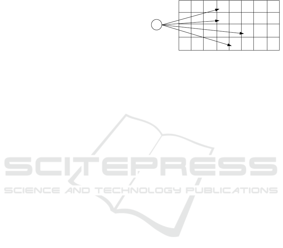
to some cell of each row of the table (Fig. 4).
count[k, h
k
(i)]← count[k, h
k
(i)]+ c
i
, k=1...d
.
(2)
i
+c
i
h
d
(i)
+c
i
+c
i
+c
i
h
1
(i)
Figure 4: Sketch Update Schema.
3. Reading (restoring) the accumulated values c
i
of element i (a
i
*
).
The restored value is calculated using the
formula:
a
i
* = min
k
count[k, h
k
(i)]
.
(3)
4. Estimation of the accuracy of the reconstructed
value a
i
*.
The obtained estimate a
i
*
bounds have the
following values (Cormode et al., 2005):
a
i
≤ a
i
* is guaranteed, here a
i
is the exact
value of accumulation,
a
i
* ≤ a
i
+ ε||a|| with probability at least 1-
δ, here ||a||
1
is the L
1
metric.
(4)
The Markov’s inequality was used to obtain the
right boundary a
i
* in (Cormode et al., 2005). It can
be large, everything depends on the accumulated
values L
1
=Σa
i
(see (4)). Source (Chen et al., 2017)
proposes to decrease the value of the L
1
metric by
subtracting from a some vector
β
with the same
values of the elements. Determining
β
requires
estimating the median of the exact values {a
i
} from
some random sample. The source (Chen et al., 2017)
does not shown how to obtain this sample. Similarly,
the right boundary a
i
*
can be large for some
distributions {a
i
}.
Let us estimate the accuracy of the restored value
differently. It is clear that if n ≤ w
⋅
d, then it makes no
sense to use a sketch. In this case, it is more
advantageous to use a vector of length n, since the
required memory is smaller and the exact
accumulation values {a
i
} are stored. Therefore, we
will assume that n > w
⋅
d.
Let us first estimate the probability that the
recovered value of a
i
*
will not coincide with the exact
value of a
i
. This is the probability that ∀k ∃(i
1
≠i)
(h
k
(i
1
)= h
k
(i)):
p=(1 – (1 – 1/w)
n-1
)
d
. (5)
IoTBDS 2021 - 6th International Conference on Internet of Things, Big Data and Security
264
The expression in the outer brackets corresponds
to the quantifier ∃, and the degree d corresponds to
the quantifier ∀.
Further using (5) we derive:
(1)/ (1)/ (1)/
12
( 1)/ ( 1)/
3
(1)/ / /
(1 ((1 1 / ) ) ) (1 )
((1 1 / ) )
nw nw nw
wn wd n wd
nwe de de
pw e
ee
−− −
−−− −−
−− − −
=− − =− =
−=
(6)
The Second Remarkable Limit was used in
transforms 1 and 3,
1) usually w≥128 (for transformation 1) and
2) e
(n-1)/w
>>1 due to n> w
⋅
d and d≥8 (for
transformation 3).
Let n = w
⋅
d+1 и d=8. Then we get p = 0.997 from
(6). Let n > w
⋅
d and w≥128 and d≥8. Then the
reconstructed value a
i
*
will not coincide with the
exact value a
i
with probability almost equal to 1. Let
us estimate the reconstruction error.
Due to the hash function (1) property, the
accumulated d⋅Σa
i
values evenly fill the cells of the
sketch matrix (see Fig. 4). On average, one cell has
(d⋅Σa
i
)/(w⋅d)= Σa
i
/w of accumulated values.
Therefore, any recovered value can be estimated as
follows:
a
i
*
= Σa
i
/w = (n⋅a
∧
)/w,
(7)
where a
∧
is {ai} average.
The relative recovery error a
i
is:
(a
i
*
-a
i
)/a
i
= (n/w)⋅(a
∧
/a
i
) - 1.
(8)
But n/w>d, d is the number of hash functions
(usually more than 8). Let a
i
not to exceed the
average. It follows from (8) that the relative recovery
error can be very large (hundreds of percent).
So, the following conclusions are made:
1. If the number of different elements in the
stream is n ≤ w⋅d, then it makes no sense to use a
sketch. In this case, it is more advantageous to use a
vector (one-dimensional numeric array) of length n.
2. If n > w⋅d, then the error in recovering the
accumulated values {a
i
} can be very large.
3 ANALYSIS LAYER
IMPLEMENTATION METHOD
IN A STREAMING DATA
PROCESSING SYSTEM
So, applying a sketch can lead to a large error in
restoring the accumulated values of elements coming
from the stream. Therefore, it is proposed to use a
vector (one-dimensional numeric array) of n length
instead of a sketch.
First, a matrix of such vectors is created (Fig. 5).
Each matrix vector corresponds to an indicator (Y
i
)
and a key (X
j
) or some combination of keys (X
k
= X
j
,
X
m
, ...). A hash table is also created for each key or
key combination.
Figure 5: Vector X.Y. update schema.
The next entry <keys X, indicators Y> comes
from the Queue Layer. There can be several keys.
The number n
Xi
is read by the key or their
combination from the corresponding i-th hash table.
It is used to update all vectors in the i-th column of
the matrix (by n
Xi
-1 offset). The value of the k-th
indicator extracted from the record is added to n
Xi
element of the vector (i, k).
A SELECT-like operator is used to read the
values accumulated in vectors inside a window
(frequencies, time, etc.). Trends of these values can
be displayed on the screen and/or accumulated in the
dataset. They can help a human operator to identify
critical system loads.
The SELECT statement specifications can be
represented as follows:
SELECT {[X
i
][,][E][{[A]X
i
.< Y
j
|*>}]}
FROM {vector (<i|*>,< j|*>)}
[WHERE {[X
i
in A
i
] [AND] [<X
i
|*>.Y
j
in B
j
]}];
(9)
The brackets {...} denote a list of items or a single
item. Brackets [...] indicate optional constructs. The
brackets <...> indicate that the separator | is used. The
indices i, j in different constructs of the select-
statement are independent. X
i
is a key or combination
of keys, Y
j
is an indicator. A
i
and B
j
are lists of values
or a single value, E is an arithmetic expression over
the elements in a list, A is an aggregate, | stands for
OR. The ‘in’ keyword can be replaced with the
arithmetic comparison operator (=,>, <, etc.).
The following attributes are used as keys and their
combinations (X):
X
1
- driver - key,
Analysis Layer Implementation Method for a Streaming Data Processing System
265

X
2
- pick-up area - key,
X
3
- (driver, pick-up area) – key combination,
X
4
- car class - key,
X
5
- car number - key,
X
6
- (driver, car number) - key combination.
The following attributes act as indicators (Y)
(possible values are indicated in brackets):
Y
1
- order served (1 or 0),
Y
2
- delivery time (time interval of the car
delivery from the moment the order is received),
Y
3
- passenger refusal (1 or 0),
Y
4
- driver refusal (1 or 0),
Y
5
- the car got into a road accident (1 or 0),
Y
6
- the car was stopped by the police (1 or 0),
Y
7
- negative feedback from the passenger (1
or 0).
The flow receives a completed order <keys,
indicators>. Key values are extracted from it: driver,
pick-up area, car class, car number (X
1
, X
2
, X
4
, X
5
).
Two key combinations are built: (driver, pick-up
area) and (driver, car number) (X
3
, X
6
). The number
n
Xi
is read from each hash table i. The n
Хi
number is
used to update the cells (by offset n
Хi
-1) of all vector
i.j (j = 1..7). In this case, the value of the indicator Y
j
is added (summed up) to the cell. If there is no
corresponding record in the hash table i, then it is
included and the number n
Xi
is assigned to it.
Below are examples of select statements that
conform to specifications (9).
1. Find the average time for a taxi driver arrival in
some area:
SELECT X
3
, X
3
.Y
2
/ X
3
.Y
1
FROM vector 3.1, vector 3.2;
(10)
All records of hash table 3 are scanned (see Figure
5). For each key X
3
= (driver, pick-up area) number
n
X3
is read. This number is used to read the values Y
2
= (delivery time) (from vector 3.2) and Y
1
= (order
served) (from vector 3.1). Division of these values is
performed. This is analogous to grouping by the X
3
composite key.
2. Display the performance indicators of all
drivers involved in a road accident:
SELECT X1.*
FROM vector 1.*
WHERE X1.Y
5
>0;
(11)
All records of hash table 1 are viewed. For each
key X
1
= (driver) number n
X1
is read. This number is
used to read the value of the Y
5
indicator. If it is
greater than 0, then all performance indicators of this
driver are output from vector 1.j, j = 1 ... 7.
Queries are executed when the window is moved.
The indicator values collected over the window time
interval are read. The following algorithm is applied:
1) put T=0, W=W
0
- the initial size of the window
(over time it can be floating),
2) reset all hash tables and vectors "vector i.j",
3) set the size of the current floating window
equal to W=t-T when the element number in the
stream is greater than n,
4) at time t =T+W, activate the program which:
- executes queries, displays current window
results, these values are added to the previous results
to obtain trends,
5) put T=t, W=W
0
, go to step 2 of the algorithm.
Web sockets can be used to access the in-memory
data store (see Data Access Layer). Upon receiving
the "slow down" command from the client (i.e. the
client is overloaded), the window size can be
automatically increased (this will reduce the λ load on
the client). The element number quantity in the
stream shall be controlled as it may become larger
than the size of the vector n (see the previous
algorithm).
Sliding window application is not feasible here.
The maintenance of hash tables and vectors on the
sliding window interval becomes much more
complicated. It would require figuring out each time
what you want to delete in hash tables and vectors
after the next sliding interval.
The vector linearity should certainly be used here.
Vectors can be updated on different servers, and then
combined on the coordinating server at the end.
The volume of vectors that are stored in the node
RAM is small. Suppose n=w⋅d=2
7
⋅2
3
=2
10
(one sketch
size). One vector volume is v1=n⋅4 (bytes) = 4KB.
Let the number of hash tables be 6 (the number of
keys and their combinations), and the number of
indicators is 7. Then the volume of all vectors in the
RAM of the node is V = 4 (KB) · 6 · 7 = 168 KB.
The proposed approach for the Analysis Layer
implementation has the following advantages:
- Select statement (9) provides greater search
capabilities than ordinary sketches (Psaltis et al.,
2017; Cormode et al., 2005; Cormode et al., 2011;
Chen et al., 2017).
- New Y parameter vectors can be included (or
excluded) dynamically.
- Hash tables with new keys or their combinations
(X) can be included (or excluded) dynamically.
- It is possible to build key combinations, which
allows executing select operators on these
combinations.
- Floating window can be used if the number of
different elements in the stream exceeds n. This saves
IoTBDS 2021 - 6th International Conference on Internet of Things, Big Data and Security
266
memory and vector updating time, since there is no
need to increase its size. The vector size should only
be dynamically increased if (1) there is an overload
on the client accessing the dataset in memory and (2)
the number of elements in the stream becomes more
than n when the window size increases.
4 EXPERIMENT
Let us compare two options for implementing the data
Analysis Layer. It is 1) a proposed vector matrix
(VM) method and 2) sketches (SK) using the Count-
Min Sketch algorithm.
Let us consider for example the “Served Taxi
Orders” subject area from Section 3.
The experiment system configuration is provided
below:
- message stream enters the system from the
Apache Kafka topic partitions;
- client-handler, coded in Go, subscribes to the
topic, processes messages, and updates the distributed
cache (Redis);
- the Redis caches are combined on one computer
with 16Gb of RAM.
Below is a record fragment example from a
stream:
{
"driver": "aa3bbae6-7c02-451f-abdc-
738c70d1544d",
…
"params": {
"time": 100,
"served": 1,
}
}
where
“driver” field – X
1
(driver) key from section 3,
“time” field – indicator Y
2
(delivery time), “served”
field –indicator Y
1
(order served).
The Y
2
value was uniformly distributed in the
range from 1 to 100 during the experiment.
For the VM method, an array of vectors was used
(see Fig. 5). To implement the SK method, the vectors
"vector i.j" in Fig. 5 was replaced with "sketch i.j".
The following query was investigated: to
determine the average time of car delivery for all
trips. Let us represent it in the form of a select
statement (see (9)):
SELECT sum X
1
.Y
2
/sum X
1
.Y
1
AS avg
FROM vector (1.2), vector (1.1);
(12)
The following parameters were changed within
the experiment:
- dc is the number of unique drivers with trips in
the time window W=1 day (key power X
1
);
- d, w is the size of one sketch;
- n is the vector size.
The VM and ES methods were evaluated
according to two criteria:
- accuracy of query execution (12);
- the amount of stored data in one sketch and
vector.
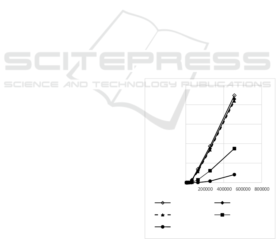
1. Query execution accuracy.
The VM method always gives an accurate result.
The SK method gives a high query execution
error (Fig. 6). With increasing ‘dc’, the error reaches
hundreds and thousands percent.
2. The volume of data stored in one sketch and
vector.
The sketch size does not depend on the cardinality
of the X
1
key (the number of different ‘dc’ values).
But with an increase in the values of the d and w
sketch parameters its volume increases (Fig. 7).
The vector size increased in proportion to the
number of unique drivers (n=dc) in the experiment.
With dc = 640,000, the amount of stored data in
the vector is less than the sketch size (d=14
w=100,000) by 5.34 / 2.44=2.2 times. At the same
time, the query execution error using a sketch reaches
200% (see Figure 6).
Figure 6: The relative error of avg recovery from a sketch.
0
500
1000
1500
2000
2500
0 500000 1000000
Relative
error, %
dc
d: 10, w: 20000 d: 14, w: 20000
d: 17, w: 20000 d: 14, w: 40000
d: 14, w: 100000
Analysis Layer Implementation Method for a Streaming Data Processing System
267
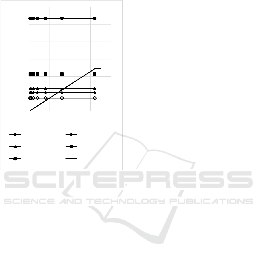
Figure 7: Storage Size Dependencies.
5 DISCUSSION
The developed VM method always wins in terms of
the query execution accuracy, but in some cases it
loses in terms of the required memory (see Fig. 7).
Section 3 suggests a way to avoid unlimited memory
growth. A floating window can be used for this. For
example, the vector size can be fixed at 2.44 MB (see
the horizontal section of the Vector row in Fig. 7).
The loss of new drivers can be avoided by reducing
the window size. At the same time, the calculations
accuracy is preserved. With dc=700,000, the window
size will automatically become equal to
W=640,000/700,000 = 0.91 days. With dc =
1,280,000, the window size will be ~50% less: W =
640,000 / 1,280,000 = 0.5 days. At the end of each
window, vectors and hash tables (see Fig. 5) are
cleared. The window size is automatically restored
and becomes equal to W=1 day. A decrease in the
window size signals an increase in the load on the
system. The human operator can track this on a
screen.
6 CONCLUSION
The sketch method was demonstrated to produce a
large error in restoring accumulated values for a
sufficiently large number of elements in a stream.
The stream data Analysis Layer structure is
proposed. It uses vectors for accumulating an
element. Unlike sketches vector arrays store accurate
aggregated values.
Vector manipulation method is proposed. It
allows dynamically include/exclude vectors and
hash-tables for new Y indicators and X keys. It is
possible to dynamically build key combinations.
A select-operator is proposed that allows
obtaining data slices by indicators and/or keys. This
increases processing flexibility compared to
traditional methods.
Floating windows size calculation algorithm is
proposed. It allows avoiding overflow of any vector
with the load increase. This increases the load λ on
the client which is processing requests to the in-
memory dataset.
The volume of vectors stored in the node RAM is
small. This allows vectors to be quickly transmitted
over the network and combined by the coordinating
server using the linearity property.
Future work includes application of the developed
data analysis tool as an Acceleration Layer in lambda
architecture systems.
REFERENCES
Basat, R. B., Friedman R., and Shahout R. (2018). "Stream
frequency over interval queries." Proceedings of the
VLDB Endowment 12.4 (2018): 433-445.
Bloom B., 1970. H. Space/time trade-offs in hash coding
with allowable errors // Communications of the ACM. –
1970. – V. 13. – № 7. – P. 422-426.
Chintapalli S. et al. (2016). Benchmarking streaming
computation engines: Storm, flink and spark streaming
// 2016 IEEE international parallel and distributed
processing symposium workshops (IPDPSW). – IEEE,
2016. – P. 1789-1792.
Cormode G. et al. (2011). Synopses for massive data:
Samples, histograms, wavelets, sketches // Foundations
and Trends® in Databases. – 2011. – Vol. 4. – № 1–3.
– P. 1-294.
Cormode G., Garofalakis M. (2005). Sketching streams
through the net: Distributed approximate query tracking
// Proceedings of the 31st international conference on
Very large data bases. – 2005. – P. 13-24.
Cormode G., Muthukrishnan S. (2005). An improved data
stream summary: the count-min sketch and its
applications // Journal of Algorithms. – 2005. – V. 55.
– №. 1. – P. 58-75.
0
1
2
3
4
5
6
0 200000 400000 600000 800000
Storage
size, Mb
dc
d: 10, w: 20000 d: 14, w: 20000
d: 17, w: 20000 d: 14, w: 40000
d: 14, w: 100000 Vector
IoTBDS 2021 - 6th International Conference on Internet of Things, Big Data and Security
268

Chen J., Zhang Q. (2017). Bias-Aware Sketches //
Proceedings of the VLDB Endowment. – 2017. – V. 10.
– № 9. – P. 961-972.
Flajolet P. et al. (2007). Hyperloglog: the analysis of a near-
optimal cardinality estimation algorithm // Conference
on Analysis of Algorithms. – 2007. - P.127–146.
Giroire F. (2005). Order statistics and estimating
cardinalities of massive data sets // International
Conference on Analysis of Algorithms DMTCS proc.
AD. – 2005. – V. 157. – P. 166.
Heule S., Nunkesser M., Hall A. (2013). HyperLogLog in
practice: algorithmic engineering of a state of the art
cardinality estimation algorithm // Proceedings of the
16th International Conference on Extending Database
Technology. – 2013. – P. 683-692.
Kroß J., Krcmar H. (2016). Modeling and simulating
apache spark streaming applications // Softwaretechnik-
Trends. – 2016. – V. 36. – №. 4. – P. 1-3.
Narkhede, N., Shapira, G. and Palino, T. (2017). Kafka: the
definitive guide: real-time data and stream processing
at scale. "O'Reilly Media, Inc.", 2017.
Noghabi S. A. et al. (2017). Samza: stateful scalable stream
processing at LinkedIn // Proceedings of the VLDB
Endowment. – 2017. – V. 10. – №. 12. – P. 1634-1645.
Poppe O., et al., 2020. "GRETA: graph-based real-time
event trend aggregation." arXiv preprint
arXiv:2010.02988 (2020).
Psaltis, A. G. (2017). Streaming Data: Understanding the
Real-Time Pipeline. Manning Publications, 2017.
Quoc D. L. et al. (2017). Approximate stream analytics in
apache flink and apache spark streaming // arXiv
preprint arXiv:1709.02946. – 2017.
Tarkoma, S., Rothenberg, C. E., and Lagerspetz, E. (2012).
Theory and practice of bloom filters for distributed
systems. IEEE Communications Surveys and Tutorials,
14(1):131–155, 2012.
Wu H., Shang Z., Wolter K. (2019). Performance
Prediction for the Apache Kafka Messaging System //
2019 IEEE 21st International Conference on High
Performance Computing and Communications; IEEE
17th International Conference on Smart City; IEEE 5th
International Conference on Data Science and Systems
(HPCC/SmartCity/DSS). – IEEE, 2019. – P. 154-161.
Yan, Yizhou, et al. (2018). "SWIFT: mining representative
patterns from large event streams." Proceedings of the
VLDB Endowment 12.3 (2018): 265-277.
Zhang, D., et al. (2018). Trajectory simplification: an
experimental study and quality analysis. in Proceedings
of the VLDB Endowment 11.9 (2018): 934-946.
Analysis Layer Implementation Method for a Streaming Data Processing System
269
