Approximate Query Processing for Lambda Architecture
Aleksey Burdakov
1a
, Uriy Grigorev
1b
, Andrey Ploutenko
2c
and Oleg Ermakov
1d
1
Bauman Moscow State Technical University, Moscow, Russia
2
Amur State University, Blagoveschensk, Russia
Keywords: Lambda Architecture, Stream Processing, Approximate Query Processing, Sapprox.
Abstract: The lambda architecture is widely used to implement streaming data processing systems. These systems create
batch views (subsets of data) at the Serving Layer to speed up queries. This operation takes significant time.
The article proposes a novel approach to lambda architecture implementation. A new method for Approximate
Query Processing in a system with Lambda Architecture (LA-AQP) significantly reduces aggregate (sum,
count, avg) calculation error. This is achieved by using a new way of calculating the reading segments
probabilities. The developed method is compared with the modern Sapprox method for processing large
distributed data. Experiments demonstrate that LA-AQP almost equals Sapprox in terms of volume and time
characteristics. The introduced accuracy measures (δ-accuracy and ε-accuracy) are up to two times better
than Sapprox for total aggregate calculation. Aggregate values can vary greatly from segment to segment. It
is shown that in this case the LA-AQP method gives a small error in the total aggregate calculation in contrast
to Sapprox.
1 INTRODUCTION
Real-time large data volume processing is an
important requirement for modern high-load systems.
Streaming data processing serves this task. Data
stream processing applies to various fields: search
engines, social networks, fraud detection systems,
trade and financial systems, equipment monitoring
systems, military and intelligence systems
(Kleppmann, 2017).
Lambda architecture enables implementation of
streaming data processing (Marz et al., 2015).
Sources (Kiran et al., 2015; Gribaudo et al., 2018)
provide lambda architecture implementation for data
processing backend in Amazon EC2. It provides high
bandwidth with low network maintenance costs. The
lambda architecture enables streaming processing
implementation in many other areas: heatmap
tracking (Perrot et al., 2017), query processing (Yang
et al., 2017), medical surgery predictions
(Spangenberg et al. 2017), etc.
a
https://orcid.org/0000-0001-6128-9897
b
https://orcid.org/0000-0001-6421-3353
c
https://orcid.org/0000-0002-4080-8683
d
https://orcid.org/0000-0002-7157-4541
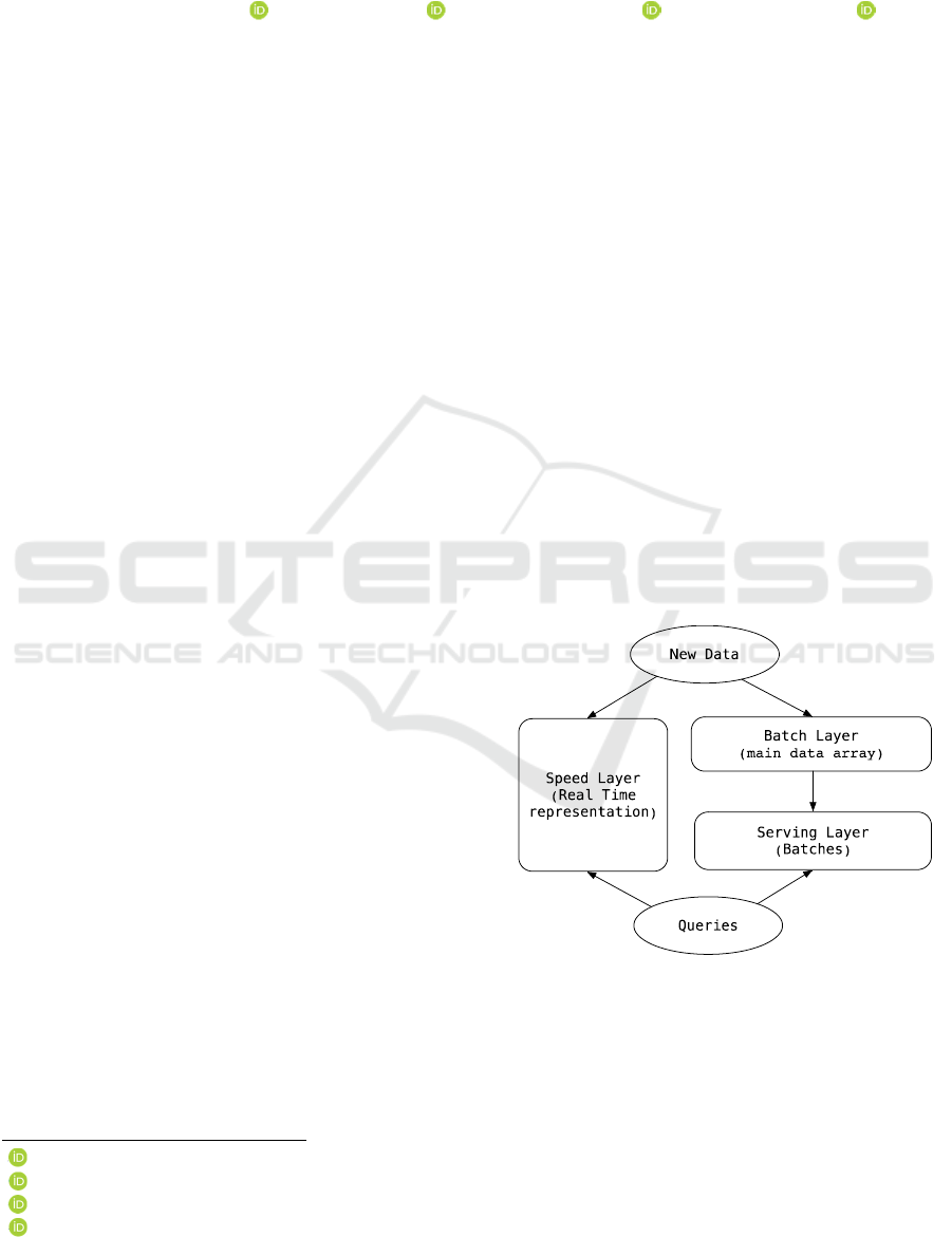
The lambda architecture (see Fig. 1 (Marz et al.,
2015)) has Batch, Speed and Serving Layers.
Figure 1: Lambda Architecture.
Apache Hadoop-based Data Lake typically
represent a Batch Processing Layer. This layer stores
a dataset master copy. The Serving Layer generates
batch representations from the data. Each batch is a
Burdakov, A., Grigorev, U., Ploutenko, A. and Ermakov, O.
Approximate Query Processing for Lambda Architecture.
DOI: 10.5220/0010465802530261
In Proceedings of the 6th International Conference on Internet of Things, Big Data and Security (IoTBDS 2021), pages 253-261
ISBN: 978-989-758-504-3
Copyright
c
2021 by SCITEPRESS – Science and Technology Publications, Lda. All rights reserved
253
data chunk prepared for fast query processing. The
Speed Layer provides real-time data processing, since
data cannot quickly reach the Serving Layer.
The described lambda architecture
implementation has a number of significant
drawbacks:
1. Effective implementation of different levels
may require different databases. This in turn requires
different development, support and data access
software tools. Source (Marz et al., 2015) provides an
example of the Batch Layer implementation based on
the Hadoop Distributed File System (HDFS), while
the Serving Layer is based on ElephantDB, and Speed
Layer uses Cassandra database.
2. A new request may require a new batch
representation (data subset). This will lead to
searching the large Batch Layer database.
3. The new data appears at the Serving Layer with
a delay. This leads to introduction of a cumbersome
Speed Layer in order to provide prompt access to such
data (Psaltis, 2017).
The article proposes a novel approach to building
systems with lambda architecture. It allows the
Serving Layer implementation in a form of metadata
describing data segments of the Batch Layer. The new
approach provides an approximate query processing
based on this metadata.
2 LAMBDA ARCHITECTURE
WITH SERVING LAYER IN
METADATA FORM
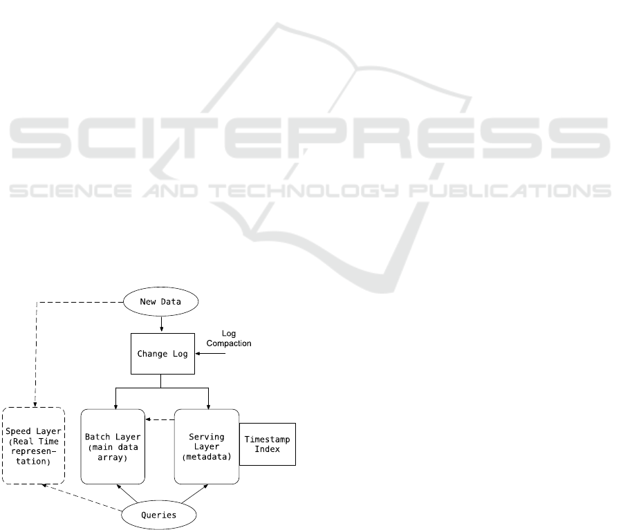
The proposed new Lambda Architecture is shown on
Fig. 2.
Figure 2: New Lambda Architecture.
First, new data blocks come from a source (e.g.
Kafka/ Storm) to the changelog. The entries in each
block are sorted by timestamp, but they are not sorted
throughout different blocks.
After a certain period of time, e.g. one second, the
background process is started. It sorts the incoming
block records by timestamp (merge sort). This
process then adds the sorted record segments to the
main dataset (Batch Layer).
The background process analyzes each record
segment. It extracts the attributes, calculates the
aggregated values, and stores them as metadata
(Serving Layer). One line of metadata corresponds to
one segment of the Batch Layer. The processed
blocks are removed from the change log (the log is
compacted), and the background process goes into a
waiting state. The new blocks received during the
execution of the background process will be
processed in the next period of this process activation.
Batch level segment records are stored as <key>
<value>, where "key" is a timestamp and "value" is a
JSON document. All records of the main data set are
sorted by key (by analogy with LSM trees based on
SS tables (Kleppmann, 2017; O’Neil, 1996)).
Metadata is used to approximate the aggregated
values (sum, avg, count) of some JSON document
attributes. As noted, one metadata record corresponds
to one segment of the Batch Layer. Metadata records
are stored as <key><value>, where “key” is the
number of the corresponding segment, “value” is a
JSON field.
The search attributes for which the search is
performed will be denoted as SA. The attributes by
which the aggregation is performed will be
designated as AA. The information for each search
attribute SA
i
is stored in the metadata record as JSON
field elements. This item has the following structure:
<k is the SA
i
value number> <number of
records in the g segment with the kth SA
i
value> {<aggregate value by the AA
m
attribute for the kth SA
i
value in the g
segment>}
m
= <Z
i
k
><M
ig
k
>{<A
igm
k
>}
m
(1)
The values of each SA
i
search attribute are stored
in a dictionary, which is common for all segments.
The dictionary is a hash table located in RAM. The
hash table elements have the following form: <SA
i
value> <k - number of SA
i
value> = < C
i
k
> <Z
i
k
>.
The dictionary is populated as new values of the
search attribute appear in the data stream when
parsing data segments. The length of a numeric field
<k - the number of the SA
i
value> is often much
shorter than the length of the character field <SA
i
IoTBDS 2021 - 6th International Conference on Internet of Things, Big Data and Security
254

value>. Therefore, the size of the metadata record
will be smaller.
The following data is additionally stored in the
metadata record:
<g-th segment timestamp> <g-th segment
number of records> <g segment number of
search attributes> {<aggregate value by
attribute AA
m
for this segment g>}
m
=
<T
g
><S
g
><Q
g
>{<A
gm
>}
m
(2)
The A
igm
k
and A
gm
aggregate values in (1) and (2)
accumulate as records are retrieved from the data
stream.
The considered lambda architecture organization
has the following advantages over the classical
scheme (see Fig. 1):
1. One database can be used to implement the
Package and Serving Layer.
2. There is no need to build batch views at the
Serving Layer. The Approximate Query Processing is
fast, and it only requires changing the view which
means only changing the SELECT query. Moreover,
aggregate values computation is usually performed at
some time interval. Having a timestamp index at the
Serving Layer allows quick reading of the required
segments from the main data set.
3. The Speed Layer is optional. For example, let
us assume that a background compaction process is
invoked every second. If the minimum statistics
collection interval is one minute, then the Speed
Layer is not needed. This Layer would be required if
statistics was collected every second.
3 RELATED WORK
Modern clusters provide enormous processing power.
But querying large-scale datasets remains
challenging. To solve this problem, approximate
calculations are used in big data analytics
environments (Laptev et al., 2012; Agarwal et al.,
2013; Pansare et al., 2011; Goiri et al., 2015; Kandula
et al., 2016).
There are various ways of dataset approximate
query processing (Cormode et al., 2011): data
sampling, histograms, wavelets.
Histogram and wavelet application presents the
following issues: 1) it is difficult to distribute data
across several nodes and process them in parallel, 2)
it is very difficult to perform the table join operation.
Therefore, the most acceptable way of
Approximate Query Processing is selecting data from
the general population. Let us consider some
methods in this area.
BlinkDB (Agarwal et al., 2013) generates patterns
on the most commonly used column sets (QCS) in
WHERE, GROUP BY, and HAVING clauses. If the
query does not match the pattern, then the aggregate
calculation error can be large. But the important thing
is that it is not possible to generate separate samples
for all data subsets.
The data sampling system ApproxHadoop (Goiri
et al., 2015) works on the assumption that the
requested datasets are evenly distributed across the
entire dataset. Unfortunately, in many real cases,
dataset subsets are actually spread unevenly across
the entire dataset partitions. The system suffers from
inefficient sampling and large variance in the
computed aggregate value.
Source (Zhang et al., 2016) proposed a more
effective method for processing large distributed data
(Sapprox method) and presented comparison results
of Approximate Query Processing in Sapprox,
ApproxHadoop and BlinkDB. The Sapprox method
was the most effective. Let us consider it in more
detail.
The Sapprox method uses the following metadata
storage structures:
1. List of attributes of the dataset table:
{<name of the search attribute of the SA
i
of the dataset table> <pointer to the hash
table with the values of the search attribute
of the SA
i
>}
i
.
2. Hash table with the search attribute SA
i
values:
{<k-th value of SA
i
> <pointer to the table
of occurrences of the k-th value of SA
i
>}
k
.
3.Table of occurrences of the k-th SA
i
value:
<k-th value of SA
i
> {<g - segment
number> <number of records in the g-th
segment with k-th value of SA
i
>}
g
=
<C
i
k
>{<g><M
ig
k
>}
g
.
4. Table of segment offsets in the HDFS
file system: {<segment number>
<segment offset in HDFS (bytes)>}
(3)
Sapprox allows approximate aggregate value
calculation (agg - sum, count) in the following
queries:
SELECT {agg(AA
m
) as A
m
}
m
FROM table
WHERE SA
1
=C
1
k1
and SA
2
=C
2
k2
and ...
and SA
h
=C
h
kh
(4)
Approximate Query Processing for Lambda Architecture
255

The algorithm is provided below:
1. For all i=1..h, g=1 ... N, calculate the
probability that the record of the g-th segment
satisfies the condition for the i-th search attribute (SA
i
= C
i
ki
): P
ig
= M
ig
ki
/S, where M
ig
ki
is the number of
records in the g-th segment with the k
i
-th value of the
SA
i
(see (3)), S is the number of records in the
segment (it is the same for all g), N is the total number
of segments in the HDFS data array.
2. For each g=1...N calculate the probability that
the record of the g-th segment satisfies the condition
specified after the WHERE keyword (see (4)):
1
h
g
ig
i
P
P
=
=
∏
3. For each g = 1 ... N calculate the probability
1
/
N
g
gj
j
P
P
π
=
=
.
4. Get a sample of 'n' segment numbers using the
probability distribution function {π
g
}.
5. Read these 'n' segments. Find records in each
segment that satisfy the WHERE clause. Calculate
the aggregated value τ
j
(j=1..n) for each AA
m
attribute
of the found records (see (4)).
6. Estimate each desired aggregate A
m
value with
the formula:
1
1
() ( )
n
j
j
j
n
n
τ
τ
π
=
=
(5)
Estimate (5) is unbiased. For a sufficiently large
‘n’ value (5) has normal distribution (Zukerman,
2020) (Lyapunov theorem). It was shown in (Liese et
al., 2008) that the random variable
t= 1 ( ( ) ) / ( )nn Dn
ττ
−⋅ −
has Student’s
distribution with n-1 degrees of freedom, where τ is
the mathematical expectation τ(n), i.e. the true value
of A
m
,
2
1
() ( ( ()))/
n
jj
j
Dn n n
τπ τ
=
=−
is an
estimate of the sample variance. We derive the
following formula:
2
1,
1
1
|()| ( ())
(1)
n
j
n
j
j
nt n
nn
α
τ
ττ τ
π
−
=
−<= −
−
,
(6)
where α is the degree of confidence of inequality
(6). For n>121 the coefficient t
n-1,
α
practically does
not depend on ‘n’, and for α=0.9; 0.95; 0.99 it is equal
to 1.645, respectively; 1,960; 2.576.
The Sapprox method has several serious
disadvantages:
1. The probability distribution {π
g
} depends only
on the probabilities {P
g
} that the segment records
satisfy the WHERE condition. This can lead to a
large estimation error if the aggregated values of τ
j
differ significantly for different segments (see the
Discussion section).
2. It is possible to calculate the aggregated
attribute values of only one table (table joins are not
supported). The search term includes elementary
terms with the logical operation 'and'. The query does
not explicitly support the GROUP BY clause.
3. When executing a query, it is necessary to read
and analyze metadata for all N segments that are
stored in the main data set (indexing by timestamps is
not supported).
4. It is necessary to read both metadata and data
segments even when a search condition is specified
for only one attribute.
5. Only HDFS file system is used, which makes it
difficult to move to other systems for storing the main
data and metadata.
6. The record number in different segments must
be the same (S). This can result in reading the same
segment from different nodes.
7. When adding a new value of the search
attribute or a new segment it is necessary to modify
the metadata created earlier (see (3)).
4 NEW APPROXIMATE QUERY
PROCESSING METHOD
Structures (1) and (2) describe metadata of the system
with the proposed lambda architecture (see Fig. 2).
These include the aggregated values calculated for
each search attribute value in the segment (A
igm
k
) and
for the segment as a whole (A
gm
). They can be
obtained by processing streaming data entering the
system.
A method of Approximate Query Processing in a
system with Lambda Architecture (LA-AQP) was
developed. It allows approximately calculation of the
aggregated values (agg - sum, count, avg) when
executing queries of the following form:
SELECT SA
r
,{agg(AA
m
) as A
m
}
m
FROM array JSON-documents
WHERE TSR and [Predicate(SA
1
,SA
2
, ...,
SA
h
)] GROUP BY SA
r
,
(7)
TSR defines timestamp search condition (time
slot, multiple time slots),
Predicate (SA
1
, SA
2
, ..., SA
h
) includes elementary
conditions for search attributes {SA
i
}, logical
operations AND, OR, NOT, and parentheses.
The low level A
igm
k
and A
gm
values are known
(see (1) and (2)). But the problem is how to use them
IoTBDS 2021 - 6th International Conference on Internet of Things, Big Data and Security
256

to quickly estimate the total aggregate A
m
in
accordance with query (7). So the A
igm
k
or A
gm
metadata values cannot be simple added because only
a part of the segment records match the WHERE
search condition. The challenge is calculating the
aggregate value that is linked to this part of the
records. The problem of estimating the number of
record parts that satisfy the search condition is also
not trivial. A probabilistic approach is used to solve
it.
The algorithms for query (7) execution are
provided below:
Algorithm 1. No predicate.
1. Read metadata records for TSR using a
timestamp index.
2. Check all found metadata records. Accumulate
the values A
m
rk
+= A
rgm
k
for each k-th value of the
search attribute SA
r
and each aggregated attribute
AA
m
(see (1)). SA
r
is an attribute by which grouping
is performed (see (7)).
Algorithm 2. Predicate is present.
1. For TSR, read metadata records using a
timestamp index.
2. For each metadata record found, calculate the
probability P
g
that the segment record satisfies the
condition specified in the Predicate. This requires the
following steps:
- calculate the probability that the segment record
satisfies the elementary condition for the i-th search
attribute (SA
i
= C
i
{ki}
): P
ig
= M
ig
{ki}
/S
g
, where C
i
{ki}
is
one or several values {k
i
} from the search dictionary
the SA
i
attribute, M
ig
{ki}
is the number of records in
the g-th segment with the values {k
i
} of the SA
i
search attribute, S
g
is the number of records in the g
segment (see (1), (2));
- calculate the probability P
g
that the record of the
g-th segment satisfies the condition specified in the
Predicate. For this one should use recursive functions
for calculating probabilities (Table 1).
Table 1: Probabilities for elementary conditions.
Condition Probability
<condition>AND<condition > <P>·<P>
<condition>OR<condition > <P>+<P>-<P>·<P>
NOT<condition> 1-<P>
P
ig
probabilities for elementary conditions
initially act as <P>.
3. Calculate the probability π
gm
for each g
segment and each aggregated attribute AA
m
:
- calculate d
gm
=(A
gm
/S
g
)·(P
g
·S
g
) - this is an
estimare of an aggregate value in the segment; indeed,
the expression in the first parentheses is an estimate
of the aggregate value per segment record (see (2));
and the expression in the second parentheses is an
estimate of the number of segment records that satisfy
the condition specified in the Predicate;
- calculate the probability
gm gm gm
{g}
π=d/ d
,
where {g} is the set of segment numbers obtained
from the read metadata.
Perform the following steps of the algorithm for
each AA
m
.
4. Get a sample of ‘n’ segment numbers {g} using
the probability distribution function {π
gm
}
g
. Sampling
should be done with repetition. Otherwise, estimate
(5) will be biased and the confidence interval
calculated using formula (6) will be erroneous.
Samples of segment numbers for different AA
m
may
have a non-empty intersection.
5. Read these 'n' segments from the main dataset.
Find JSON documents in each segment that satisfy
the condition specified in the Predicate. Calculate the
aggregated value τ
j
(j = 1..n) for them for the AA
m
attribute (ie select the AA
m
values from JSON
documents). For each k-th value of the SA
r
search
attribute, accumulate the values A
m
rk
+= AA
m
jrk
.
6. Estimate the aggregated A
m
value (without
grouping) using the formula (5). Calculate the
confidence interval using formula (6). The confidence
interval for the group aggregate A
m
rk
(see clause 5)
does not exceed this value. This is derived from the
fact that the variance D(n) for A
m
is equal to the sum
of the variances calculated for A
m
rk
.
The LA-AQP method has the following
advantages:
1. The confidence interval, calculated using the
formula (6), decreases. The quantity d
jm
/π
jm
(see item
3 of Algorithm 2) is some approximation of the
quantity τ
j
/π
j
in D (n) (see (6)). Since
jm jm gm
{g}
d/π= d
these relationships are the
same for different j. Therefore, the variance D (n) can
be expected to be smaller.
2. It is not necessary to read segments from the
main data set of the Batch Layer to obtain the result
in some important cases (see Algorithm 1).
3. An arbitrary Predicate for search attributes of
JSON documents and use the GROUP BY clause (see
(7)) can be specified in a query.
4. There is a timestamp index that allows reducing
the number of analyzed metadata records and,
thereby, reducing the sample size.
5. The number of S
g
JSON documents in the
segments can be different (see (2)).
6. The old metadata records are not changed when
new records are added during the data stream
processing.
Approximate Query Processing for Lambda Architecture
257
7. Different distributed file systems (not
necessarily HDFS) can be used to implement the
method. The required segments of the main dataset
are read at offset.
8. There is no need to develop a method for
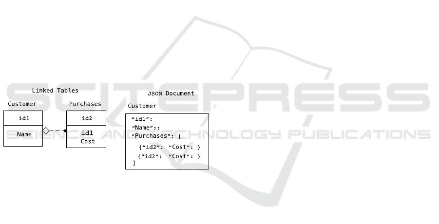
related tables approximate query processing.
Suppose it is necessary to approximately process the
following query:
SELECT sum(Cost) FROM Customer T1,
Purchases T2 WHERE T1.id1=T2.id1 AND Name=
“José”.
If linked tables are used (Figure 3, left), then the
tables "Customer" and "Purchases" need to be split
into segments. Let their number be N1 and N2
respectively. In further processing, it is necessary to
consider pairs of segments in order to take into
account the relationship of segments by the common
attribute id1. The number of such pairs (new
segments) equals N1×N2.
The JSON document stores all information
related to the client (see Figure 3, right). So that the
tables were already joined by the id1 attribute in these
documents. In this case, the number of segments is
reduced to N1.
Figure 3: Related tables and the corresponding structure of
the JSON document.
5 COMPARISON OF SAPPROX
AND LA-AQP APPROXIMATE
QUERY PROCESSING
METHODS
The comparison was carried out on a computer with
a four-core processor and 16 GB RAM. Testing of
Sapprox and LA-AQP methods was done on synthetic
dataset. The system received a stream of financial
transactions in JSON format. Each document
included the following fields:
- sum is the payment amount (random value from
0 to 10,000),
- city is the client's city (one of 1000 random
cities),
- user_id is the id of a specific client (one of
1,000,000 random user IDs),
- factor is deposit / withdrawal (one of 2 values),
- a variable number of additional fields.
Outlying peak values were generated to simulate
the trend of increasing payments in different cities.
They did not coincide with the distribution function
of payment amounts at the previous points in time.
The developed system prototype consists of three
main components: balancer, database, and
multithreaded daemon for segment processing.
The balancer splits the incoming JSON
documents into segments and writes them to the
database (Data table).
The database is implemented with PostgreSQL
DBMS. Each segment is an inheritor of the base table.
Each new segment is a separate table where JSON
documents are stored. Segment reading performs
read operation of the blocks associated with the table.
Metadata is stored in a separate table. This table key
is the segment index, and the value is a JSON field.
The value is saved in the metadata instead of the
search attribute value number for the LA-AQP
method. The dictionary was not implemented in the
developed prototype. It also stores aggregated values
for search attributes and for the segment as a whole
(see (1), (2)).
The multithreaded daemon scans for new
database segments. It starts the process of building
metadata for these segments (generates metadata
records). The balancer and daemon were written in
the Golang (Go) language, which was chosen due to
the ease of writing asynchronous code (Donovan et
al., 2015; Cox-Buday et al., 2017).
68 million records (JSON documents) were
generated for the test, the segment size was set to
S=10,000 records. The following query was tested
(no timestamp constraints):
SELECT sum(Data.sum)
FROM Data
WHERE city = ‘City_1’ and factor =
‘Expense’;
(8)
The experiments were repeated 3 times for each
method and each sample size (10% and 30%).
Table 2 shows the averaged volume-time
characteristics of SQL (exact execution of the query
(8)), as well as the Sapprox and LA-AQP methods.
According to these data, the Sapprox and LA-AQP
methods performed on par.
IoTBDS 2021 - 6th International Conference on Internet of Things, Big Data and Security
258

Table 2: The averaged volume-time characteristics of SQL
for Sapprox and LA-AQP methods.
Characteristic SQL Sapprox LA-AQP
LA-AQP/
Sapprox
Difference
Time to
include one
segment
(10,000
records) into
the database
(ms)
242 373 384 +3%
Time to build
metadata for
one segment
(ms)
31 31 0%
Request
execution
time (ms)
33,372
Request
execution
time (ms),
sample size
10%
1,132 1,143 +1%
Request
execution
time (ms),
sample size
30%
2,833 2,847 +0,5%
Total database
size (GB)
12 12 12 0%
Table 3 shows the characteristics of the sum
aggregate calculation accuracy. The accuracy was
evaluated in two ways:
1. δ=max (1-L/E, U/E-1),
where L is the lower limit of the calculated
aggregate; E is the aggregate exact value; U is the
upper bound of the calculated aggregate.
2. ε is the value of the confidence interval (this is
the doubled value of the right-hand side of inequality
(6)) divided by 5,000. The exact value of the
aggregate sum divided by 5,000 is 63,014,300/5,000
= 12,603.
Table 3 demonstrates that the developed LA-AQP
method is almost two times better in δ-accuracy than
the Sapprox method. Moreover, the LA-AQP method
with a 10% sample is better in δ-accuracy than the
Sapprox method with a 30% sample. In terms of ε-
accuracy, the LA-AQP method is almost 1.8≈2 times
better than Sapprox.
Table 3: The characteristics of the sum aggregate
calculation accuracy.
Characteristic Sapprox LA-AQP
LA-AQP
difference
from
Sapprox
δ, 10% sample
volume
0.12 0.07 -42%
δ, 30% sample
volume
0.09 0.04 -56%
ε, 10% sample
volume,
α=0,9/0,95/0,99
1209/1440/1896 704/838/1106 -42%
ε, 30% sample
volume,
α=0,9/0,95/0,99
1050/1253/1647 544/648/847 -48%
6 DISCUSSION
In the developed LA-AQP method, when calculating
the probabilities π
gm
, the values of the aggregates in
the segment are taken into account. This is the
fundamental difference between LA-AQP and
Sapprox as well as other methods. As shown in
Section 4, this allows reducing the confidence
interval (6) when estimating τ.
The aggregated values of τ
j
can differ
significantly for different segments. The Sapprox
method in this case can lead to a large estimation error
τ. Let us give a small example.
Let the number of segments be N=2000 and the
sample size n=100. Suppose that P
g
=0.1, g = 1 ... N,
i.e. 10% of the records in each segment satisfy the
WHERE search condition. Let the aggregated values
τ
j
of any attribute of these records be distributed over
segments significantly unevenly: τ
1
= 10000, τ
j
=1, j=2
... 2000.
Then for Sapprox π
g
= P
g
/(N⋅ P
g
)=0.0005, g = 1 ...
N (see item 3 of the algorithm in Section 3). The
probability that in n = 100 trials the 1st segment will
not be selected equals (1-π
1
)
n
=0,95. From formula
(5), we obtain an aggregate estimate:
1st option - 1st segment is not selected:
τ(n)=(1/n)⋅n⋅((τ
j
=1)/(π
j
=0.0005)=2,000;
2nd option - 1st segment will be selected with
probability 1-0.95 = 0.05:
τ(n)=(1/n)⋅( (τ
1
=10,000)/π
1
+(n-1)⋅(τ
j
=1)/π
j
)=
201,980.
Approximate Query Processing for Lambda Architecture
259

In fact τ=(τ
1
=10,000)+(N-1)⋅(τ
j
=1)=11,999. The
estimation error τ is large in options 1 and 2.
Let us show that with the same initial data, the
LA-AQP method allows estimating τ with a much
smaller error. In this case, we obtain (see item 3 of the
algorithm 2 in Section 4):
π
1
=((τ
1
=10,000)⋅P
1
)/
((τ
1
=10,000)⋅P
1
+ (N-1)⋅(τ
j
=1)⋅P
j
)= 0.83;
π
j
=((τ
j
=1)⋅P
j
)/
((τ
1
=10,000)⋅P
1
+(N-1)⋅(τ
j
=1)⋅P
j
)=8.33E-5, j=2...N.
The probability that for n=100 trials the 1st
segment will not be selected is (1-π
1
)
n
=1.1E-77 (i.e.
it is practically 0). We derive an aggregate value
estimate from formula (5):
Option 1 - the 1st segment will be selected only
one time out of n = 100:
τ(n)=(1/n)⋅((τ
1
=10,000)/
π
1
+(n-1)⋅(τ
j
=1)/π
j
)=12,005;
Option 2 - the 1st segment will be selected 100
times out of n=100:
τ(n)=(1/n)⋅(n⋅(τ
1
=10,000)/π
1
)= 12,048.
Option 3 - the 1st segment is not selected (this is
an almost impossible event):
τ(n)=(1/n)⋅(n⋅(τ
j
=1)/π
j
)= 12,004.
Therefore the error in calculating the aggregate is
small (exact value τ=11,999) in options 1, 2 and 3 for
LA-AQP. The sample size 'n' is not important in this
example, and it can be equal to one. It also does not
matter which segment numbers are selected for
processing. The calculation error using the LA-AQP
method will be small in any case.
To achieve the same level of error in Sapprox,
it is necessary to significantly increase the sample
size n. It should be comparable to N.
The LA-AQP method allows specifying a more
complex search condition and a GROUP BY clause
in a query (see (7)). Sapprox allows only AND (see
(4)) connection of elementary conditions.
7 CONCLUSIONS
The existing systems with lambda-architecture
requires constantly repeat package updates for new
analytical queries execution acceleration. This
consumes large time since it searches in a large
database. The developed approach allows avoiding
creation of package representations due to the
introduction of metadata level. The queries are
executed promptly but with a certain error. The
developed LA-AQP method reduces this error.
Expression (5) gives an unbiased estimate of the
τ aggregate for any probability distribution function
{π
g
}, π
g
>0. The issue is in the sample size. The
developed method for calculating {π
g
} makes it
possible to obtain a good aggregate estimation
accuracy for small n values. This is achieved due to
the fact that when calculating {π
g
}, estimates of the
values of the aggregates in the segment are used. As
a result, the values τ
j
/π
j
in (5) become approximately
the same. This allows minimizing the sample
variance D(n) (see (6)).
The LA-AQP method allows executing queries
with a general search condition and with a grouping
(see (7)). For calculations, aggregate values are used
at the level of individual attributes and segments. The
overhead costs of obtaining such aggregates are low:
they accumulate as data arrives in the stream. The
accuracy of the general aggregates increases
approximately twofold as compared with the Sapprox
method.
The future work includes development a method
for processing queries at the Speed Layer in a Lambda
Architecture system.
REFERENCES
Agarwal, S., Mozafari, B., Panda, A., Milner, H., Madden,
S., and Stoica, I. (2013). Blinkdb: Queries with
bounded errors and bounded response times on very
large data. In Proceedings of the 8th ACM European
Conference on Computer Systems, EuroSys ’13, pages
29–42, New York, NY, USA, 2013. ACM.
Cormode, G. et al. (2011). Synopses for massive data:
Samples, histograms, wavelets, sketches // Foundations
and Trends® in Databases. – 2011. – Vol. 4. – №. 1–3.
– P. 1-294.
Cox-Buday, K. (2017). Concurrency in Go: Tools and
Techniques for Developers. "O'Reilly Media, Inc.",
2017.
Donovan, Alan AA, and Kernighan B. W. (2015). The Go
programming language. Addison-Wesley Professional,
2015.
Gribaudo, M., Iacono, M., Kiran M. A. (2018).
Performance modeling framework for lambda
architecture based applications // Future Generation
Computer Systems. – 2018. – Vol. 86. – pp. 1032-1041.
Goiri, R., Bianchini, S., Nagarakatte and Nguyen, T. D.
(2015). Approxhadoop: Bringing approximations to
mapreduce frameworks. In Proceedings of the
Twentieth International Conference on Architectural
Support for Programming Languages and Operating
IoTBDS 2021 - 6th International Conference on Internet of Things, Big Data and Security
260

Systems, ASPLOS ’15, pages 383–397, New York, NY,
USA, 2015. ACM.
Kandula, S., Shanbhag, A., Vitorovic, A., Olma, M.,
Grandl, R., Chaudhuri, S. and Ding, B. (2016). Quickr:
Lazily approximating complex adhoc queries in bigdata
clusters. In Proceedings of the 2016 ACM SIGMOD
International Conference on Management of Data,
SIGMOD ’16, New York, NY, USA, 2016. ACM.
Kiran, M. et al. (2015). Lambda architecture for cost-
effective batch and speed big data processing // 2015
IEEE International Conference on Big Data (Big
Data). – IEEE, 2015. – pp. 2785-2792.
Kleppmann, M. (2017). Designing data-intensive
applications: The big ideas behind reliable, scalable,
and maintainable systems. "O'Reilly Media, Inc.",
2017.
Laptev, N., Zeng, K. and Zaniolo, C. (2012). Early accurate
results for advanced analytics on mapreduce. Proc.
VLDB Endow., 5(10):1028–1039, June 2012.
Liese, F., Miescke, K.J. (2008). Statistical Decision Theory
Estimation, Testing, and Selection. Springer Series in
Statistics, 2008.
Marz, N., and James W. (2015). Big Data: Principles and
best practices of scalable real-time data systems. New
York; Manning Publications Co., 2015.
O’Neil, P. et al. (1996). "The log-structured merge-tree
(LSM-tree)." Acta Informatica 33.4 (1996): 351-385.
Pansare, N., Borkar, V. R., Jermaine, C., and Condie, T.
(2011). Online aggregation for large mapreduce jobs.
Proc. VLDB Endow, 4(11):1135–1145, 2011.
Perrot, A. et al. (2017). HeatPipe: High Throughput, Low
Latency Big Data Heatmap with Spark Streaming //
2017 21st International Conference Information
Visualisation (IV). – IEEE, 2017. – pp. 66-71.
Psaltis, A. G. (2017). Streaming Data: Understanding the
Real-Time Pipeline. Manning Publications, 2017.
Spangenberg, N., Wilke M., Franczyk B., 2017. A Big Data
architecture for intra-surgical remaining time
predictions // Procedia computer science. – 2017. –
Vol. 113. – pp. 310-317.
Yang, F. et al. (2017). The RADStack: Open source lambda
architecture for interactive analytics // Proceedings of
the 50th Hawaii International Conference on System
Sciences. – 2017. - pp. 1703-1712.
Zhang, X., Wang, J., Yin, J. (2016). Sapprox: enabling
efficient and accurate approximations on sub-datasets
with distribution-aware online sampling // Proceedings
of the VLDB Endowment. – 2016. – V. 10. – №. 3. – pp.
109-120.
Zukerman, M. (2020). Introduction to Queueing Theory
and Stochastic Teletrac Models. [Online]. Available:
http://www.ee.cityu.edu.hk/~zukerman/classnotes.pdf.
[Accessed: Sept. 22, 2020]
Approximate Query Processing for Lambda Architecture
261
