A Practical Guide to Support Predictive Tasks in Data Science

Jos

e Augusto C

amara Filho

, Jos

e Maria Monteiro

, C

esar Lincoln Mattos

and Juv

encio Santos Nobre

Department of Computing, Federal University of Cear

a, Fortaleza, Cear

a, Brazil

Department of Statistics and Applied Mathematics, Federal University of Cear

a, Fortaleza, Cear

a, Brazil

Keywords:

Practical Guide, Prediction, Data Science.

Abstract:

Currently, professionals from the most diverse areas of knowledge need to explore their data repositories in

order to extract knowledge and create new products or services. Several tools have been proposed in order

to facilitate the tasks involved in the Data Science lifecycle. However, such tools require their users to have

speciﬁc (and deep) knowledge in different areas of Computing and Statistics, making their use practically

unfeasible for non-specialist professionals in data science. In this paper, we propose a guideline to support

predictive tasks in data science. In addition to being useful for non-experts in Data Science, the proposed

guideline can support data scientists, data engineers or programmers which are starting to deal with predic-

tive tasks. Besides, we present a tool, called DSAdvisor, which follows the stages of the proposed guideline.

DSAdvisor aims to encourage non-expert users to build machine learning models to solve predictive tasks, ex-

tracting knowledge from their own data repositories. More speciﬁcally, DSAdvisor guides these professionals

in predictive tasks involving regression and classiﬁcation.

1 INTRODUCTION

Due to a large amount of data currently available,

arises the need for professionals of different areas to

extract knowledge from their repositories to create

new products and services. For example, cardiolo-

gists need to explore large repositories of electrocar-

diographic signals in order to predict the likelihood

of sudden death in a certain patient. Likewise, tax

auditors may want to explore their databases in or-

der to predict the likelihood of tax evasion. How-

ever, in order to build predictive models, these non-

specialist professionals need to acquire knowledge in

different areas of Computing and Statistics, making

this task practically unfeasible. Another alternative

is ask experienced data science professionals to help,

which creates dependency instead of autonomy. In

this context, the popularization of data science be-

comes an important research problem (Provost and

Fawcett, 2013).

Data science is a multidisciplinary area involv-

ing the extraction of information and knowledge from

large data repositories (Provost and Fawcett, 2013).

It deals with the data collection, integration, manage-

ment, exploration and knowledge extraction to make

decisions, understand the past and the present, pre-

dict the future, and create new services and prod-

ucts (Ozdemir, 2016). Data science makes it pos-

sible to identifying patterns hidden and obtain new

insights hidden in these datasets, from complex ma-

chine learning algorithms.

The Data Science lifecycle has six stages: busi-

ness grasp, data understanding, data preparation,

modeling, evaluation, and deployment. To extract

knowledge from the data, we must be able to (i) un-

derstand yet unsolved problems with the use of data

mining techniques, (ii) understand the data and their

interrelationships, (iii) extract a data subset, (iv) cre-

ate machine learning models in order to solve the se-

lected problem, (v) evaluate the performance of the

new models, and (vi) demonstrate how these models

can be used in decision-making (Chertchom, 2018).

The complexity of the previous tasks explains why

only highly experienced users can master the entire

Data Science lifecycle. On the other hand, several

tools have been proposed in order to support the tasks

involved in the Data Science lifecycle. However, such

tools require their users to have speciﬁc (and deep)

knowledge in different areas of Computing and Statis-

tics, making their use practically unfeasible for non-

specialist professionals in data science.

In this paper, we propose a guideline to support

248

Filho, J., Monteiro, J., Mattos, C. and Nobre, J.

A Practical Guide to Support Predictive Tasks in Data Science.

DOI: 10.5220/0010460202480255

In Proceedings of the 23rd International Conference on Enter prise Information Systems (ICEIS 2021) - Volume 1, pages 248-255

ISBN: 978-989-758-509-8

predictive tasks in data science. In addition to being

useful for non-experts in Data Science, the proposed

guideline can support data scientists, data engineers

or programmers which are starting to deal with pre-

dictive tasks. In addition, we present a tool, called

DSAdvisor, which following the stages of the pro-

posed guideline. DSAdvisor aims to encourage non-

expert users to build machine learning models to solve

regression or classiﬁcation tasks, extracting knowl-

edge from their own data repositories. DSAdvisor

acts like an advisor for non-expert users or novice data

scientists.

The rest of this paper is organized as follows. Sec-

tion 2 reviews related works. In section 3, the pro-

posed guideline is laid out. The DSAdvisor is com-

mented in section 4. Finally, in section 5 we present

our conclusions and suggestions for future research.

2 RELATED WORKS

In this section we will discuss the main related works.

For a better understanding, we organized the related

works into two categories: supporting tools and prac-

tical guidelines.

2.1 Data Mining Tools

Traditional data mining tools help companies estab-

lish data patterns and trends by using a number of

complex algorithms and techniques. As example of

such tools, we can cite: KEEL, Knime, Orange,

RapidMiner and WEKA (Hasim and Haris, 2015).

KEEL (Knowledge Extraction based on Evolu-

tionary Learning) is a software that facilitates the

analysis of the behavior of evolutionary learning in

different approaches of learning algorithm such as

Pittsburgh, Michigan, IRL (iterative rule learning)

and GCCL (genetic cooperative-competitive learn-

ing) (Alcal

a-Fdez et al., 2009). Knime is a mod-

ular environment that enables easy integration of

new algorithms, data manipulation and visualization

methods. It allows the selection of different data

sources, data preprocessing steps, machine learning

algorithms, as well as visualization tools. To cre-

ate the workﬂow, the user drag some nodes, drop

onto the workbench, and link it to join the input

and output ports. The Orange tool has different

features which are visually represented by widgets

(e.g. read ﬁle, discretize, train SVM classiﬁer, etc.).

Each widget has a short description within the in-

terface. Programming is performed by placing wid-

gets on the canvas and connecting their inputs and

outputs (Dem

sar et al., 2013). RapidMiner pro-

vides a visual and user friendly GUI environment.

This tool uses the process concept. A process may

contain subprocesses. Processes contain operators

which are represented by visual components. An

application wizard provides prebuilt workﬂows for

a number of common tasks including direct market-

ing, predictive maintenance, sentiment analysis, and a

statistic view which provides many statistical graphs

(Jovic et al., 2014). Weka offers four operating op-

tions: command-line interface (CLI), Explorer, Ex-

perimenter and Knowledge ﬂow. The “Explorer” op-

tion allows the deﬁnition of data source, data prepa-

ration, run machine learning algorithms, and data vi-

sualization (Hall et al., 2009). DSAdvisor is an ad-

visor for non-expert users or novice data scientists,

which following the stages of the guideline proposed

in this paper. DSAdvisor aims to encourage non-

expert users to build machine learning models to solve

regression or classiﬁcation tasks, extracting knowl-

edge from their own data repositories.

Even before the popularization of data Science,

all these tools were developed to help with data min-

ing tasks. These tools differ regarding tool usability,

type of license, the language in which they were de-

veloped, support for data understanding, and missing

values handle. The most widely used tools include

KEEL, Knime, Orange, RapidMiner, Tanagra, and

Weka. The table 1 provides a comparison between

these tools and the DSAdvisor.

In the other hand, AutoML tools enable you to au-

tomate some machine learning tasks. Although it be

important to automate all machine learning tasks, that

is not what AutoML does. Rather, it focuses on a few

repetitive tasks, such as: hyperparameter optimiza-

tion, feature selection, and model selection. Exam-

ples of these tools include: AutoKeras, Auto-WEKA,

Auto-Sklearn, DataRobot, H20 and MLBox.

2.2 Guidelines

A guideline is a roadmap determining the course of a

set of actions that make up a speciﬁc process, in addi-

tion to a set of good practices for the performance of

these activities (Dictionary, 2015). Some guidelines

have been proposed to manage general data mining

tasks.

In (Melo et al., 2019), the authors presented a

practical guideline to support the speciﬁc problem of

predict change-proneness classes in oriented object

software. In addition, they applied their guideline

over a case study using a large imbalanced dataset ex-

tracted from a wide commercial software. It is im-

portant to highlight that, in this work, we extend the

A Practical Guide to Support Predictive Tasks in Data Science

249

Table 1: General characteristics of data mining software. Adapted from (Hasim and Haris, 2015).

Softwares list

Software Usability License Language Data Understanding Missing values handle

DSAdvisor High GPL Python Perform Intermediate

KEEL High GPL Java Perform Basic

KNIME Low Outra Java Perform Basic

RapidMiner High GPL Java Partially performs Basic

Orange Low GPL C++, Python Partially performs Basic

Weka Low GPL Java Partially performs Basic

guideline proposed in (Melo et al., 2019) to the more

general data science context.

(Luo et al., 2016) highlight the ﬂexibility of

the emerging machine learning techniques, however,

there is uncertainty and inconsistency in the use of

such techniques. Machine learning, due to its intrin-

sic mathematical and algorithmic complexity, is often

considered “black magic” that requires a delicate bal-

ance of a large number of conﬂicting factors. This, to-

gether with inadequate reporting of data sources and

the modeling process, makes the research results re-

ported in many biomedical articles difﬁcult to inter-

pret. It is not uncommon to see potentially spurious

conclusions drawn from methodologically inadequate

studies, which in turn undermines the credibility of

other valid studies and discourages many researchers

who could beneﬁt from adopting machine learning

techniques. In the light of this, guidelines are pro-

posed for the use of predictive models in clinical set-

tings, ensuring that activities are carried out correctly

and reported.

3 THE PROPOSED GUIDELINE

FOR PREDICTIVE TASKS

This section describes the proposed guide to support

regression and classiﬁcation tasks, which is organized

into three phases: exploratory analysis, data prepro-

cessing and building predictive models. Each one of

these phases will be detailed next.

3.1 Phase 1: Exploratory Analysis

The ﬁrst phase of the proposed guideline aims to ana-

lyze a dataset, provided by the user, and next, describe

and summarize it. Figure 1 illustrates this phase,

which comprises the following activities: uploading

the data, checking the type of variables, removing

variables, choosing missing value codes, exhibiting

descriptive statistics, plotting categorical and discrete

variables, analyzing distributions, and displaying cor-

relations.

So, the guide indicates the use of different descrip-

tive statistics, such as the number of lines (count),

mean, standard deviation (std), coefﬁcient of varia-

tion (cv), minimum (min), percentiles (25%, 50%,

75%) and maximum (max) for numerical variables,

and count, number of distinct values (unique), the

most frequent element (top) and the most common

value’s frequency (freq) for categorical variables. Be-

sides, the guideline recommend the use of different

strategies for identifying and showing missing values.

Moreover, the proposed guideline suggests dif-

ferent methods to assess the distribution of vari-

ables, such as Cram

er Von Mises (Cram

er, 1928),

D’Agostino’s K-squared (D’Agostino, 1970), Lil-

liefors (Lilliefors, 1967), Shapiro-Wilk (Shapiro and

Wilk, 1965) and Kolmogorov-Smirnov (Smirnov,

1948). All these methods serve to determine the ve-

racity of a hypothesis (Hirakata et al., 2019). In

this guide we want to state whether a variable fol-

lows (H0) or not (H1) a normal distribution, and each

method has its own way of calculating and return-

ing a result to identify the most suitable hypothesis.

Each test considers two hypotheses about the variable

under study. One is called the null hypothesis (H0),

which is assumed to be true until proven otherwise.

The second is called the alternative hypothesis (H1),

which represents a statement that the parameter of in-

terest differs from that deﬁned in the null hypothesis,

so that the two hypotheses are complementary. The

hypotheses used by the tests are: i)H0: The variable

follows a normal distribution and ii) H1: The variable

does not follow a normal distribution.

Finally, the guide indicates the use of different

correlation coefﬁcients based on the data distribution.

Spearman’s correlation coefﬁcients (Spearman, 1961)

will be displayed for all pair of numerical data. If a

pair of variables (columns or features) follow a nor-

mal distribution, the Pearson’s correlation coefﬁcients

(Pearson, 1895) must be computed and shown. If the

user dataset contains categorical data, the guide sug-

gest to display Cramer’s V. (Cram

er, 1928).

ICEIS 2021 - 23rd International Conference on Enterprise Information Systems

250

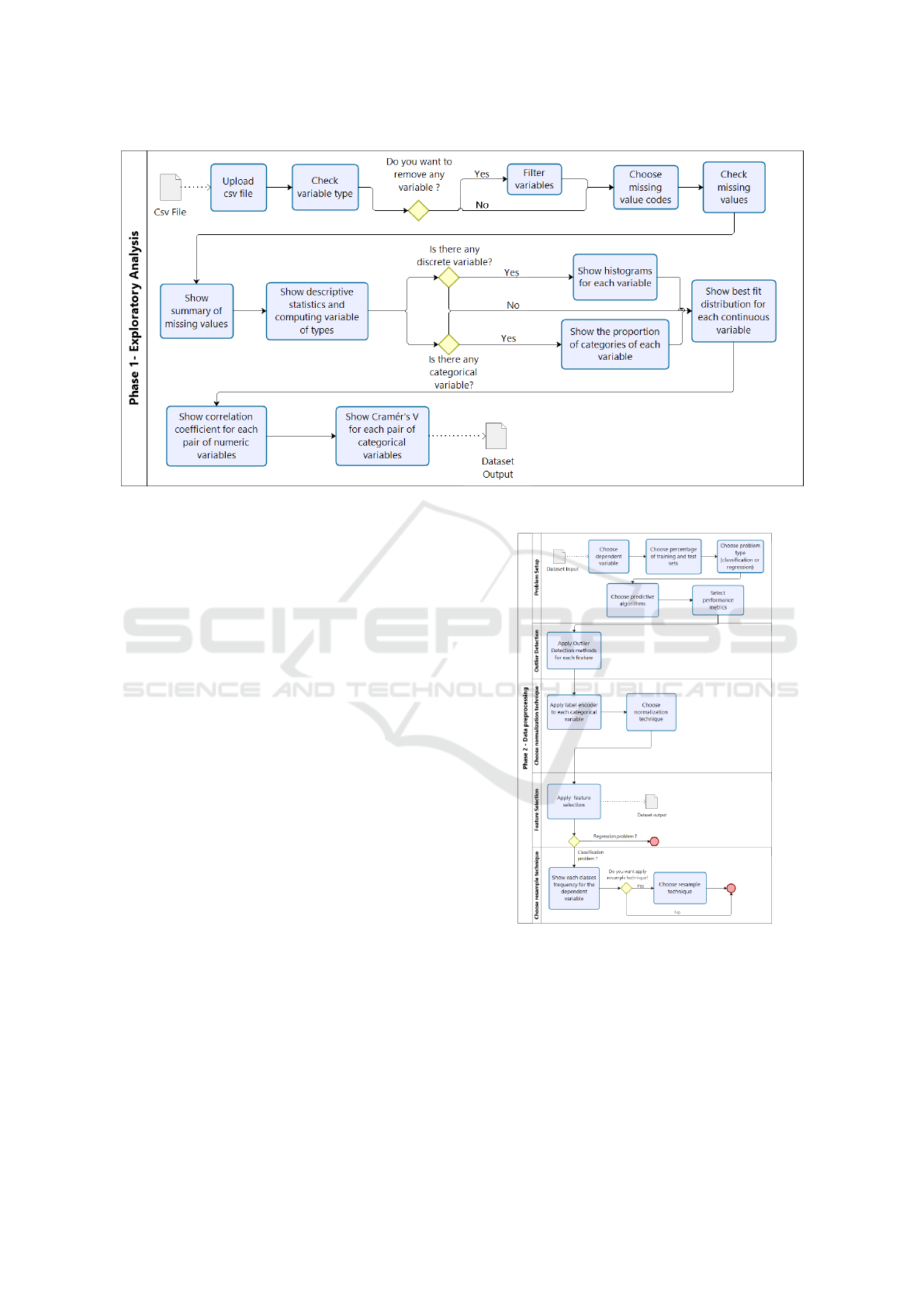
Figure 1: Phase 1 - Exploratory Analysis.

3.2 Phase 2: Data Preprocessing

Data preprocessing is an essential component to solve

many predictive tasks. The purpose of the second

phase of the proposed guide is to prepare the data

in order to use it to build predictive models. This

phase includes activities related to outlier detection,

data normalization, choose the independent variable,

selection of attributes, data balancing, feature selec-

tion, and division of training and testing sets. Figure 2

illustrates the activities that make up the second phase

of the proposed guide.

3.2.1 Problem Setup

In this step, the predictive task type (regression or

classiﬁcation) must be deﬁned. Besides, the depen-

dent variable should be identiﬁed. Moreover, the pro-

portion of the training and test sets have to be spec-

iﬁed. Other options for the third phase are the pre-

dictive algorithms list, score function for optimizing

GridSearchCV and metrics list for Results Presenta-

tion. The list of predictive algorithms, the list of met-

rics and the score function will be according to the

type of problem to be treated, classiﬁcation’s or re-

gression’s problem.

3.2.2 Choose Normalization Techniques

Verifying that the variables are on the same scale is

an essential step at this point. For example, two vari-

ables may be expressed in different ranges, such as

integers and the interval between 0 and 1. Therefore,

Figure 2: Phase 2 - Data preprocessing.

it is necessary to normalize all variables in the dataset.

For instance, for the activation function in the neural

network it is recommended that the data be normal-

ized between 0.1 and 0.9 instead of 0 and 1 to avoid

saturation of the sigmoid function (Basheer and Ha-

jmeer, 2000). The normalization techniques used in

this guideline are z-score and min-max normalization.

A Practical Guide to Support Predictive Tasks in Data Science

251

3.2.3 Outlier Detection

Outliers are extreme values that deviate from other

observations on data (i.e., an observation that diverges

from an overall pattern on a sample). Detected out-

liers are candidates for aberrant data that may other-

wise adversely lead to model misspeciﬁcation, biased

parameter estimation and incorrect results. It is there-

fore important to identify them prior to creating the

prediction model (Liu et al., 2004).

A survey to distinguish between univariate vs.

multivariate techniques and parametric (Statistical)

vs. nonparametric procedures was done by (Ben-

Gal, 2005). Detecting outliers is possible when multi-

variate analysis is performed and the combinations of

variables are compared with the class of data. In other

words, an instance can be a multivariate outlier but a

usual value in each feature, or it can have values that

are outliers in several features, but the whole instance

might also be a usual multivariate value (Escalante,

2005).

There are two main techniques to detect outliers:

interquartile range (a univariate parametric approach)

and adjusted boxplot (a univariate nonparametric ap-

proach). Next, we describe each one of these tech-

niques.

Interquartile Range. The interquartile range (IQR)

is a measure of statistical dispersion, often used to

detect outliers. The IQR is the length of the box

in the boxplot (i.e., Q3 - Q1). Here, outliers are

deﬁned as instances below Q1 − 1.5 ∗ IQR or above

Q3 + 1.5 ∗ IQR.

Adjusted Boxplot. Note that the boxplot assumes

symmetry because we add the same amount to Q3 as

we subtract from Q1. In asymmetric distributions, the

usual boxplot typically ﬂags many regular data points

as outlying. The skewness-adjusted boxplot corrects

that by using a robust measure of skewness in deter-

mining the fence (Hubert and Vandervieren, 2008). In

this new approach, outliers are deﬁned as instances

such that if medcouple (MC) ≥ 0, they are below

Q1 − 1.5e

−4mc

∗ IQR or above Q1 + 1.5e

3mc

∗ IQR;

if not, they are below Q1 − 1.5e

−3mc

∗ IQR or above

Q1 + 1.5e

4mc

∗ IQR. To measure the skewness of a

univariate sample (x

, ... , x

) from a continuous uni-

modal distribution F, we use the MC, and Q2 is the

sample median (Brys et al., 2004). It is deﬁned as in

equation 1:

MC = med

≤Q2≤x

h(x

, x

) (1)

Outliers are one of the main problems when building

a predictive model. Indeed, they cause data scientists

to achieve suboptimal results. To solve that, we need

effective methods to deal with spurious points. If it is

obvious that the outlier is due to incorrectly entered

or measured data, you should drop the outlier.

3.2.4 Feature Selection

Feature selection is referred to the process of obtain-

ing a subset from an original feature set according to

certain feature selection criterion, which selects the

relevant features of the dataset. It plays a role in com-

pressing the data processing scale, where the redun-

dant and irrelevant features are removed (Cai et al.,

2018). Feature selection technique can pre-process

learning algorithms, and good feature selection re-

sults can improve learning accuracy, reduce learning

time, simplify learning results, reduction of dimen-

sional space and removal of redundant, irrelevant or

noisy data (Ladha and Deepa, 2011).

Feature selection methods fall into three cate-

gories: ﬁlters, wrappers, and embedded/hybrid meth-

ods. Filter method takes less computational time

for selecting the best features. As the correlation

between the independent variables is not considered

while selecting the features, this leads to selection of

redundant features (Venkatesh and Anuradha, 2019).

Wrapper are brute-force feature selection methods

that exhaustively evaluate all possible combinations

of the input features to ﬁnd the best subset. Embed-

ded/hybrid methods combine the advantages of both

approaches, ﬁlters and wrappers. A hybrid approach

uses both performance evaluation function of the fea-

ture subset and independent test. (Veerabhadrappa

and Rangarajan, 2010).

3.2.5 Choose Resample Techniques for

Imbalanced Data

Imbalanced data problem occurs in many real-world

datasets where the class distributions of data are asi-

metric. It is important to note that most machine

learning models work best when the number of in-

stances of each class is approximately equal (Lon-

gadge and Dongre, 2013). The imbalanced data prob-

lem causes the majority class to dominate the minor-

ity class; hence, the classiﬁers are more inclined to

the majority class, and their performance cannot be

reliable (Kotsiantis et al., 2006).

Many strategies have been generated to handle the

imbalanced data problem. The sampling-based ap-

proach is one of the most effective methods that can

solve this problem. The sampling-based approach

can be classiﬁed into three categories, namely: Over-

Sampling (Yap et al., 2014), Under-Sampling (Liu

et al., 2008), and Hybrid Methods (Gulati, 2020). In

this guide we recommend the use of over-sampling

and under-sampling.

ICEIS 2021 - 23rd International Conference on Enterprise Information Systems

252

Over-sampling (OS). Over-sampling raises the

weight of the minority class by replicating or creat-

ing new minority class samples. There are different

over-sampling methods; moreover, it is worth noting

that the over-sampling approach is generally applied

more frequently than other approaches.

• Random Over Sampler: This method increases

the size of the dataset by the repetition of the orig-

inal samples. The point is that the random over-

sampler does not create new samples, and the va-

riety of samples does not change (Li et al., 2013).

• Smote: This method is a statistical technique that

increases the number of minority samples in the

dataset by generating new instances. This algo-

rithm takes samples of the feature space for each

target class and its nearest neighbors, and then

creates new samples that combine features of the

target case with features of its neighbors. The new

instances are not copies of existing minority sam-

ples (Chawla et al., 2002).

Under-sampling (US). Under-sampling is one of the

most straightforward strategies to handle the imbal-

anced data problem. This method under-samples the

majority class to balance the class with the minority

class. The under-sampling method is applied when

the amount of collected data is sufﬁcient. There

are different under-sampling models, such as Edited

Nearest Neighbors (ENN) (Guan et al., 2009), Ran-

dom Under-Sampler (RUS) (Batista et al., 2004) and

Tomek links (Elhassan and Aljurf, 2016), which are

the most popular.

3.3 Phase 3: Building Predictive Models

This phase aims to generate predictive models and

analyze their results. For this purpose we introduce

pipeline, pipeline is a Sklearn class (Pedregosa et al.,

2011) to sequentially apply a list of transformations

and ﬁnal estimator on a dataset. Pipeline objects

chain multiple estimators into a single one. This is

useful since a machine learning workﬂow typically

involves a ﬁxed sequence of processing steps (e.g.,

feature extraction, dimensionality reduction, learn-

ing and making predictions), many of which perform

some kind of learning. A sequence of N such steps

can be combined into a pipeline if the ﬁrst N − 1

steps are transformers; the last can be either a predic-

tor, a transformer or both (Buitinck et al., 2013). For

evaluating statistical performance in pipeline, we use

a GridSearch with K-Fold Cross Validation. Cross-

validation is a resampling procedure used to evaluate

machine learning models on a limited data sample.

K-fold Cross-Validation involves randomly dividing

the set of observations into k groups, or folds, of ap-

proximately equal size. The ﬁrst fold is treated as a

validation set, and the method is ﬁt on the remaining

k − 1 folds. For example, using the mean squared er-

ror as score function, MSE

, is then computed on the

observations in the held-out fold. This procedure is

repeated k times; each time, a different group of ob-

servations is treated as a validation set. This process

results in k estimates of the test error, MSE

, MSE

,..., MSE

. The K-Fold Cross-Validation estimate is

computed by averaging these values (James et al.,

2013). In our case, we focus on making predictions in

the data set for classiﬁcation and regression tasks, our

models will have the algorithms chosen by the user

according to the task to be performed. In order to

compare the models’ performance, it is necessary to

use suitable metrics. After running the pipeline, just

take the metrics previously chosen by the user to be

calculated and presented to the user in an explana-

tory way about each selected metric. The last step

in this phase consists in ensuring the experiment’s re-

producibility in order to verify the credibility of the

proposed study. (Olorisade et al., 2017) have evalu-

ated studies in order to highlight the difﬁculty of re-

producing most of the works in state-of-art. Some au-

thors have proposed basic rules for reproducible com-

putational research, as (Sandve et al., 2013), based on

these rules we save all the decisions made by the user,

the results obtained whether they are tables or graphs,

the seed and settings of the algorithms used, all in a

ﬁnal document. Figure 3 illustrates the activities that

make up the third phase of the proposed guide.

Figure 3: Phase 3 - Building Predictive Models.

4 DSAdvisor

DSAdvisor is an advisor for non-expert users or

novice data scientists, which following the stages

of the guideline proposed in this paper. DSAdvi-

sor aims to encourage non-expert users to build ma-

chine learning models to solve predictive tasks (re-

gression or classiﬁcation), extracting knowledge from

their own data repositories. This tool was developed

in CSS3, HTML5, Flask (Grinberg, 2018), JavaScript

A Practical Guide to Support Predictive Tasks in Data Science

253

and Python (van Rossum, 1995).

DSAdvisor is an open source tool, developed us-

ing the Python programming language. So, this make

possible to reuse the large number of Python APIs

and Toolkis currently available. Besides, DSAdvi-

sor provides different resources to support data un-

derstanding and missing values detection. In addic-

tion, DSAdvisor guide the user on the task of out-

lier detection showing the number of instances, the

percentage of outliers found and the total of outliers.

If the user wishes to know precisely what these val-

ues are, they can go to the outliers table option to

check the position and value of the outliers for each

variable. Furthermore, the DSAdvisor tool help the

user on the feature selection task, running the follow-

ing ﬁlters methods: Chi Squared, Information Gain,

Mutual Info, F-Value and Gain Ratio. In order to

tackle the imbalanced data problem, DSAdvisor sup-

ports three alternatives: Oversampling, Undersam-

pling and Without resampling techniques. To assess

which type of problem is being addressed (classiﬁca-

tion or regression), DSAdvisor asks some questions to

the user. Next, based on the user responses, DSAdvi-

sor suggests the most apropriate problem type. In case

of choosing classiﬁcation, the pre-selected algorithms

will be logistic regression, naive bayes, support vec-

tor machine, decision tree, and multi layer perceptron.

In case of choosing regression, the pre-selected algo-

rithms will be linear regression, support vector ma-

chine, multi layer perceptron, radial basis function.

After this, DSAdvisor suggest the most suitable per-

formance metrics. Finally, the user has the option to

download the execution log of all the options selected

previously, the results obtained whether they are ta-

bles or graphs, and the settings of all used algorithms.

This option ensures that the experiments performed in

the DSAdvisor tool are reproducible by other users.

5 CONCLUSIONS AND FUTURE

WORKS

In this paper, we propose a guideline to support pre-

dictive tasks in data science. In addition, we present

a tool, called DSAdvisor, which following the stages

of the proposed guideline. DSAdvisor aims to en-

courage non-expert users to build machine learning

models to solve predictive tasks, extracting knowl-

edge from their own data repositories. More specif-

ically, DSAdvisor guides these professionals in pre-

dictive tasks involving regression and classiﬁcation.

As future works we intent to carry out usability tests

and interviews with non-expert users, in order to eval-

uate DSAdvisor.

REFERENCES

Alcal

a-Fdez, J., Sanchez, L., Garcia, S., del Jesus, M. J.,

Ventura, S., Garrell, J. M., Otero, J., Romero, C., Bac-

ardit, J., Rivas, V. M., et al. (2009). Keel: a software

tool to assess evolutionary algorithms for data mining

problems. Soft Computing, 13(3):307–318.

Basheer, I. and Hajmeer, M. (2000). Artiﬁcial neural net-

works: fundamentals, computing, design, and appli-

cation. Journal of Microbiological Methods, 43(1):3

– 31. Neural Computting in Micrbiology.

Batista, G., Prati, R., and Monard, M.-C. (2004). A study of

the behavior of several methods for balancing machine

learning training data. SIGKDD Explorations, 6:20–

29.

Ben-Gal, I. (2005). Outlier Detection, pages 131–146.

Springer US, Boston, MA.

Brys, G., Hubert, M., and Struyf, A. (2004). A robust

measure of skewness. Journal of Computational and

Graphical Statistics, 13(4):996–1017.

Buitinck, L., Louppe, G., Blondel, M., Pedregosa, F.,

Mueller, A., Grisel, O., Niculae, V., Prettenhofer, P.,

Gramfort, A., Grobler, J., et al. (2013). Api design

for machine learning software: experiences from the

scikit-learn project. arXiv preprint arXiv:1309.0238.

Cai, J., Luo, J., Wang, S., and Yang, S. (2018). Feature se-

lection in machine learning: A new perspective. Neu-

rocomputing, 300:70–79.

Chawla, N. V., Bowyer, K. W., Hall, L. O., and Kegelmeyer,

W. P. (2002). Smote: synthetic minority over-

sampling technique. Journal of artiﬁcial intelligence

research, 16:321–357.

Chertchom, P. (2018). A comparison study between data

mining tools over regression methods: Recommenda-

tion for smes. In 2018 5th International Conference

on Business and Industrial Research (ICBIR), pages

46–50. IEEE.

Cram

er, H. (1928). On the composition of elementary er-

rors: First paper: Mathematical deductions. Scandi-

navian Actuarial Journal, 1928(1):13–74.

D’Agostino, R. B. (1970). Transformation to normality of

the null distribution of g1. Biometrika, pages 679–

681.

Dem

sar, J., Curk, T., Erjavec, A., Gorup,

C., Ho

cevar, T.,

Milutinovi

c, M., Mo

zina, M., Polajnar, M., Toplak,

M., Stari

c, A., et al. (2013). Orange: data mining

toolbox in python. the Journal of machine Learning

research, 14(1):2349–2353.

Dictionary, C. (2015). Cambridge dictionaries online.

Elhassan, T. and Aljurf, M. (2016). Classiﬁcation of imbal-

ance data using tomek link (t-link) combined with ran-

dom under-sampling (rus) as a data reduction method.

Escalante, H. J. (2005). A comparison of outlier detection

algorithms for machine learning. Programming and

Computer Software.

Grinberg, M. (2018). Flask web development: develop-

ing web applications with python. ” O’Reilly Media,

Inc.”.

Guan, D., Yuan, W., Lee, Y.-K., and Lee, S. (2009). Nearest

neighbor editing aided by unlabeled data. Information

Sciences, 179(13):2273–2282.

ICEIS 2021 - 23rd International Conference on Enterprise Information Systems

254

Gulati, P. (2020). Hybrid resampling technique to tackle the

imbalanced classiﬁcation problem.

Hall, M., Frank, E., Holmes, G., Pfahringer, B., Reutemann,

P., and Witten, I. H. (2009). The weka data min-

ing software: an update. ACM SIGKDD explorations

newsletter, 11(1):10–18.

Hasim, N. and Haris, N. A. (2015). A study of open-source

data mining tools for forecasting. In Proceedings of

the 9th International Conference on Ubiquitous Infor-

mation Management and Communication, pages 1–4.

Hirakata, V. N., Mancuso, A. C. B., and Castro, S. M. d. J.

(2019). Teste de hip

oteses: perguntas que voc

e sem-

pre quis fazer, mas nunca teve coragem. Teste de

hip

oteses: perguntas que voc

e sempre quis fazer, mas

nunca teve coragem. Vol. 39, n. 2, 2019, p. 181-185.

Hubert, M. and Vandervieren, E. (2008). An adjusted box-

plot for skewed distributions. Computational statistics

& data analysis, 52(12):5186–5201.

James, G., Witten, D., Hastie, T., and Tibshirani, R. (2013).

An introduction to statistical learning, volume 112.

Springer.

Jovic, A., Brkic, K., and Bogunovic, N. (2014). An

overview of free software tools for general data min-

ing. In 2014 37th International Convention on In-

formation and Communication Technology, Electron-

ics and Microelectronics (MIPRO), pages 1112–1117.

IEEE.

Kotsiantis, S., Kanellopoulos, D., Pintelas, P., et al. (2006).

Handling imbalanced datasets: A review. GESTS In-

ternational Transactions on Computer Science and

Engineering, 30(1):25–36.

Ladha, L. and Deepa, T. (2011). Feature selection methods

and algorithms. International Journal on Computer

Science and Engineering.

Li, H., Li, J., Chang, P.-C., and Sun, J. (2013). Paramet-

ric prediction on default risk of chinese listed tourism

companies by using random oversampling, isomap,

and locally linear embeddings on imbalanced sam-

ples. International Journal of Hospitality Manage-

ment, 35:141–151.

Lilliefors, H. W. (1967). On the kolmogorov-smirnov

test for normality with mean and variance un-

known. Journal of the American statistical Associa-

tion, 62(318):399–402.

Liu, H., Shah, S., and Jiang, W. (2004). On-line outlier

detection and data cleaning. Computers & Chemical

Engineering, 28(9):1635 – 1647.

Liu, X.-Y., Wu, J., and Zhou, Z.-H. (2008). Exploratory

undersampling for class-imbalance learning. IEEE

Transactions on Systems, Man, and Cybernetics, Part

B (Cybernetics), 39(2):539–550.

Longadge, R. and Dongre, S. (2013). Class imbal-

ance problem in data mining review. arXiv preprint

arXiv:1305.1707.

Luo, W., Phung, D., Tran, T., Gupta, S., Rana, S., Kar-

makar, C., Shilton, A., Yearwood, J., Dimitrova, N.,

Ho, T. B., et al. (2016). Guidelines for developing

and reporting machine learning predictive models in

biomedical research: a multidisciplinary view. Jour-

nal of medical Internet research, 18(12):e323.

Melo, C. S., da Cruz, M. M. L., Martins, A. D. F., Matos,

T., da Silva Monteiro Filho, J. M., and de Cas-

tro Machado, J. (2019). A practical guide to sup-

port change-proneness prediction. In ICEIS (2), pages

269–276.

Olorisade, B. K., Brereton, P., and Andras, P. (2017). Re-

producibility in machine learning-based studies: An

example of text mining.

Ozdemir, S. (2016). Principles of data science. Packt Pub-

lishing Ltd.

Pearson, K. (1895). Notes on regression and inheritance in

the case of two parents proceedings of the royal soci-

ety of london, 58, 240-242.

Pedregosa, F., Varoquaux, G., Gramfort, A., Michel, V.,

Thirion, B., Grisel, O., Blondel, M., Prettenhofer, P.,

Weiss, R., Dubourg, V., et al. (2011). Scikit-learn:

Machine learning in python. the Journal of machine

Learning research, 12:2825–2830.

Provost, F. and Fawcett, T. (2013). Data science and its rela-

tionship to big data and data-driven decision making.

Big data, 1(1):51–59.

Sandve, G. K., Nekrutenko, A., Taylor, J., and Hovig, E.

(2013). Ten simple rules for reproducible computa-

tional research. PLoS Comput Biol, 9(10):e1003285.

Shapiro, S. S. and Wilk, M. B. (1965). An analysis

of variance test for normality (complete samples).

Biometrika, 52(3/4):591–611.

Smirnov, N. (1948). Table for estimating the goodness of ﬁt

of empirical distributions. The annals of mathematical

statistics, 19(2):279–281.

Spearman, C. (1961). The proof and measurement of asso-

ciation between two things.

van Rossum, G. (1995). Python tutorial. Technical Report

CS-R9526, Centrum voor Wiskunde en Informatica

(CWI), Amsterdam.

Veerabhadrappa and Rangarajan, L. (2010). Bi-level di-

mensionality reduction methods using feature selec-

tion and feature extraction. International Journal of

Computer Applications, 4.

Venkatesh, B. and Anuradha, J. (2019). A review of feature

selection and its methods. Cybernetics and Informa-

tion Technologies, 19(1):3–26.

Yap, B. W., Abd Rani, K., Abd Rahman, H. A., Fong, S.,

Khairudin, Z., and Abdullah, N. N. (2014). An appli-

cation of oversampling, undersampling, bagging and

boosting in handling imbalanced datasets. In Pro-

ceedings of the ﬁrst international conference on ad-

vanced data and information engineering (DaEng-

2013), pages 13–22. Springer.

A Practical Guide to Support Predictive Tasks in Data Science

255