SPOT: Toward a Decision Guidance System for Uniﬁed Product

and Service Network Design

Joost Bottenbley

and Alexander Brodsky

Department of Computer Science, George Mason University, 4400 University Dr., Fairfax, Virginia, U.S.A.

Keywords:

Decision Support, Decision Guidance, Optimization, Manufacturing, Supply Chain, Product Design, Service

Network.

Abstract:

A major deﬁciency in the manufacturing ecosystem today is the lack of cloud-based infrastructure that sup-

ports the combined decision making and optimization of product design, process design, and supply chain,

as opposed to hard wired solutions within silos today. The reported work makes a step toward bridging this

deﬁciency by developing a software framework, prototype and a case study for SPOT - a decision guidance

system for simultaneous optimization and trade-off analysis of combined service and product networks, capa-

ble to express the combined product, process and supply chain design. SPOT allows users to express, as data

input, a hierarchical assembly and composition virtual products and services, i.e., having ﬁxed and control pa-

rameters that can be optimized. Virtual services produce a ﬂow of virtual products, such as raw materials, parts

of ﬁnished products. Like the virtual services, they are associated with analytic models that express customer-

facing performance metrics and feasibility constraints, which are used for optimization. The uniqueness of

our approach in SPOT is the use of modular simulation-like model for product and service networks, yet

optimization quality and computational time of the best available mathematical programming solvers, which

is achieved by symbolic computation of simulation code to generate lower-level mathematical programming

models.

1 INTRODUCTION

Smart manufacturing can be deﬁned as “the synthe-

sis of advanced manufacturing capabilities and digi-

tal technologies to improve the productivity, agility,

and sustainability of manufacturing systems” (Helu

and Hedberg, 2015). By leveraging the large amount

of data from IoT devices and real time analytics,

smart manufacturing has become a key element in

reducing manufacturing costs, improved efﬁciency,

and time-to-market (KLE, ). These reductions have

been prevalent enough for some companies to move

outsourced manufacturing services back to domestic

markets (Shehadi, 2019).

A key approach to realize a manufacturing ecosys-

tem is to employ cloud-based infrastructure that sup-

ports decision making and optimization of product de-

sign, process design, and supply chain (Brodsky et al.,

2017). Such infrastructure must support a wide vari-

ety of analytic tasks across the entire organizational

hierarchy. This includes manufacturing units, cells,

https://orcid.org/0000-0003-1702-9718

https://orcid.org/0000-0002-0312-2105

production lines, factories, and supply chains (Sal-

vendy, 2001). Considering the plethora of potential

players across an enterprise’s supply chain, it is crit-

ical “to effectively and efﬁciently combine manufac-

turing services ... [in] multiple-factory production en-

vironments” (Wu et al., 2013). Developing tools and

methods for service composition remains an on-going

research area and requires generic and robust model

representations to perform advanced analysis, e.g. op-

timization (Wu et al., 2013).

There has been extensive work on decision mak-

ing in product design (e.g., see overview (Klingstam

and Gullander, 1999)), process design (e.g., see

overview (Stoll, 1986)) and supply chain (e.g., see

overview (Garcia and You, 2015)). However, this

work is typically done in “silos”. Product design does

not take into account manufacturing process design

and supply chain. Whereas, often small modiﬁcations

in product design may result in improving manufac-

turability and costs with little or no negative effect on

customer-facing product characteristics (Eddy et al.,

2015; Herrmann et al., 2004). Similarly, manufactur-

ing process design assumes that the product design is

Bottenbley, J. and Brodsky, A.

SPOT: Toward a Decision Guidance System for Uniﬁed Product and Service Network Design.

DOI: 10.5220/0010459707170728

In Proceedings of the 23rd International Conference on Enterprise Information Systems (ICEIS 2021) - Volume 1, pages 717-728

ISBN: 978-989-758-509-8

717

already ﬁxed, limiting design choices, and does not

take into account supply chain opportunities. In turn,

during supply chain design, both product and pro-

cess design are assumed ﬁxed, limiting possibly at-

tractive sourcing options. Some work on product de-

sign (Molcho et al., 2008), did consider manufactura-

bility. However, this was used as a separate layer of

design ﬁltering, as opposed to a comprehensive com-

bined optimization.

As described in (Brodsky et al., 2017), analy-

sis and optimization solutions in manufacturing are

typically implemented from scratch, following a lin-

ear methodology (McLean and Shao, 2003; Denkena

et al., 2007). This leads to high-cost and long-

duration development and results in models that are

difﬁcult to modify, extend and reuse. This is be-

cause different computational tools, i.e., for simula-

tion and optimization, use different low-level mathe-

matical abstractions, which results in re-modeling the

same knowledge multiple times.

The work (Brodsky et al., 2016; Brodsky et al.,

2017; Brodsky et al., 2019) bridged this deﬁciency,

and also uniﬁed optimization of manufacturing pro-

cesses and supply chain by developing a software ar-

chitecture and Web-based solution called Factory Op-

tima. This tool allows manufacturers to compose, op-

timize, and perform trade-off analysis of service net-

works involving both unit manufacturing processes

and supply chains. However, their work assumes that

product design (for raw materials, part, and ﬁnished

products) is ﬁxed.

This problem is studied in (Brodsky et al., 2019),

which proposed the concept and market place for vir-

tual things (i.e. virtual products and virtual services)

based on uniﬁed modeling, analysis, and simulta-

neous optimization of product, process, and supply

chain design. However, that work is limited to a the-

oretical framework, and leaves open the problem of

developing generalized models and systems that can

support the theoretical framework.

This paper makes the ﬁrst step on bridging this

gap. More speciﬁcally, the contribution of this paper

is two-fold. First, we develop a software prototype for

SPOT

- a decision guidance system for simultane-

ous optimization and trade-off analysis of combined

service and product networks, capable to express the

combined product, process and supply chain design

toward the vision of virtual products and services of

(Brodsky et al., 2021). SPOT is based on extending

the software framework of Factory Optima (Brodsky

et al., 2016; Brodsky et al., 2017; Brodsky et al.,

2019) with a model for steady-state virtual service

and product (VSP) network which allows users to ex-

SPOT: Services and Products Optimization Tool.

press, as data input, a hierarchical assembly of prod-

ucts and composition of services in terms of (compos-

ite or atomic) sub-services. Virtual services produce

a ﬂow of virtual products (e.g., raw materials, parts

of ﬁnished products), which are, like the virtual ser-

vices, are parameterized with ﬁxed and control vari-

ables that effect product and service customer-facing

performance metrics and feasibility constraints. The

uniqueness of our approach in SPOT (like in Fac-

tory Optima) is the use of modular simulation-like

model for product and service networks, yet opti-

mization quality and computational time of the best

available mathematical programming solvers, which

is achieved by symbolic computation of simulation

code to generate lower-level mathematical program-

ming models. Second, we demonstrate SPOT on a

case study of a (virtual) bicycle product and service

network, and describe a typical methodology of its

use.

This paper is organized as follows. Section 2 pro-

vides an illustration of how SPOT translates a supply

chain network which yields any number of products

into a V-Service network and a V-Product. In addi-

tion, it describes how this V-Things can be used to

answer questions about the viability of manufactur-

ing the product. Section 3 describes the enterprise

architecture of SPOT, functionalities, common do-

main users, and types of actionable recommendations

SPOT can provide to these domain users. Section 4

provides the formal model of the problem statement,

the valid input data structure, the valid output data

structure, and the computation of the analytic model.

Section 5 demonstrates how domain users can gener-

ate a valid input data structure, set the optimization

parameters and constraints, and interpret the results.

Section 6 details the results of the study and future

research directions of interest.

2 VIRTUAL PRODUCT &

SERVICE ILLUSTRATION

As described in (Brodsky et al., 2021), a VSP, intu-

itively, is represented by a parameterized CAD de-

sign, e.g., to characterize a customizable consumer

product, part or raw material. A VSP represents a

parameterized transformation of virtual products into

other VSPs, e.g., to characterize a customizable man-

ufacturing process, supply, transportation, logistics or

a composed service network.

Each V-thing—product or service—is associated

with an analytic model that describes the product

and/or service’s feasibility and customer-facing met-

rics/characteristics as a function of the product and/or

ICEIS 2021 - 23rd International Conference on Enterprise Information Systems

718

service’s (ﬁxed and decision) parameters. For V-

products, examples of customer-facing metrics in-

clude external dimensions, weight, durability and

vacuum efﬁciency; while examples of internal param-

eters include internal dimensions, position of ﬁxtures,

and type and properties of materials. For V-services,

examples of customer-facing metrics include cost-

per-unit, total ordered quantities per item, delivery

time, carbon emissions per unit, and default risk;

while examples of internal parameters include set-

tings for unit manufacturing processes (e.g., CNC ma-

chining, injection molding or 3D printing) and se-

lection of and ordered quantities from suppliers and

manufacturers.

Intuitively, V-things’ customer-facing metrics are

all that customers care about when selecting products

and services; whereas, customers do not care about, or

even understand, V-thing parameters outside the set of

customer-facing metrics. Mathematically, an analytic

model for a V-thing - product or services — represents

a mapping from the parametric space (the input) into

the customer-facing metric space (the output.)

In order to create V-services, we focus in this pa-

per on the model development for a V-service net-

work, which allows hierarchical composition of both

v-services and V-products, recursively, out of sub-

services and sub-products. Based on this model, the

SPOT system will make actionable recommendations

on the optimal parameter instantiation of V-service

and products.

Before deﬁning a formal analytic model in Sec-

tion 4 for a VSP network, consider the example a

special bicycle production depicted in Figure 2. The

overall bicycle service network in the example in-

volves supply (depicted on the left), manufacturing

(depicted in the middle) and transportation (depicted

at the top).

Within the supply part, there are ﬁve potential sup-

pliers - including Zoltek and Tradewell LTC - which

supply raw materials such as leather, raw steel, and

plastic.

We will follow the products made by Tradewell

LTC and Zoltek to illustrate the ﬂow of material

through the supply chain. As illustrated in Figure

?? Zoltek has two outFlows: CarbonFiber01 and

Leather01. These ﬂow ids are listed in Zoltek’s out-

Flows object. Querying the ﬂows object at the top-

level will reveal that these ﬂows contain the products

carbon ﬁber and leather. In turn, querying the prod-

ucts object at the top-level provides physical charac-

teristics of the products. For example, the product ob-

ject carbon ﬁber has characteristics such as: strength

to weight ratio, rigidity, ﬁber type, thickness dry, ﬁber

areal weight, and density. As indicated by Figure

2, Zoltek’s outFlow is given to Swift Transpiration.

This agent, a atomic Transportation service (L2), pro-

vides transpiration services from Zoltek’s location to

Bianchi’s location. The location information is stored

in our shared object at the top-level so that any func-

tion can access this data.

Bianchi Corp. is a tier three (L3) manufacturer.

Unlike Suppliers, manufactures require products from

other agents within the supply chain network to pro-

duce products. In this instance, Bianchi requires car-

bon ﬁber and leather, as well as other products from

with in the supply chain, to make two products: a car-

bon ﬁber frame and a leather seat. These two products

are transported by the transportation service Fed Ex to

the ﬁnal assembly location where they are ﬁnally as-

sembled into a road bike.

Tradewell LTC also is an atomic supplier. The

outFlow id of Tradewell LTC is AU01 and con-

tains the product aluminum scrap. This product

is transported to Simurgh Iron Company through

the transportation service Create Carrier Corporation.

Simurgh Iron Company provides the service of manu-

facturing aluminum billets from raw aluminum scrap.

Simurgh Iron is a tier 2 (L2) manufacturer. West-

ern Express transports this output to Garmin, ENVE,

Bianchi, and Shimano. These tier three (L3) manu-

factures use the aluminum to create there respective

products as illustrated in Figure ??. The ﬁnal assem-

bly location receives its inputs from Fed Ex. Each of

these products are considered basic products. Basic

products are distinguished from assembled products

in the fact basic products do not require assembly.

The ﬁnal assembly service constructs the road bike

from the required parts listed in its list of components.

Now consider the decision making problem pre-

sented to investors, entrepreneurs, business develop-

ers, and other participants in the supply chain. There

are several critical decision points these stakehold-

ers would be interested in which could be easily an-

swered by this schematic of the Virtual Bicycle. En-

trepreneurs, who may have a considerable amount of

domain knowledge of their particular industry, but

no knowledge of manufacturing processes, would be

aided in their decision to contract with particular

providers of supplies and services. Business devel-

opers, who’s main focus is to maintain and develop

new relationships, would be informed about new mar-

ket participants. Investors would have considerable

knowledge about the VSPs cost, time-to-market, reg-

ulation requirements, and other KPIs that would be

stored in the library of models stored in SPOT’s model

repository.

SPOT: Toward a Decision Guidance System for Uniﬁed Product and Service Network Design

719

3 SPOT DECISION GUIDANCE

FUNCTIONALITY & SYSTEM

ARCHITECTURE

The developed SPOT Decision Guidance System is

designed to provide actionable recommendations on

optimal V-services and products instances to domain

users including entrepreneurs, investors, product &

process Designers, and supply chain analysts as well

as to CAD/CAM systems.

SPOT is a middleware software application that

facilitates the design of new VSPs by modifying

and linking existing VSPs. It enables the simul-

taneous optimization of products and services by

leveraging product-design-compositions and service-

network-compositions. In addition, it allows decision

guidance analytics in the form of performance metric

prediction, Pareto trade-off analysis, and model cali-

bration (training) using historical examples. Finally,

it supports an extensible reusable repository of VSPs

and analytic models which enable creation of a mar-

ket of VSPs.

The architecture of the DGS system is illustrated

in Figure 1. SPOT will reside on a local, centralized,

or distributed compute server and receive the neces-

sary processing request and structured data. Domain

users will submit analytic queries and receive answers

through the modeling and analytics GUI - see top

layer of Figure 1. CAD and CAM software tools can

also submit jobs to SPOT through APIs and interface

mappers.

Instead of implementing analytics functionality

using low-level analytics tools such as optimization,

simulation and machine learning (the lower layer in

Figure 1), SPOT uses the middleware of reusable, ex-

tensible, modular knowledge base of analytic mod-

els and the Decision Guidance Management System

(DGMS). Each analytic model in the KB describes

a function that, given ﬁxed and control parameters

of service and product network, computes its perfor-

mance metrics such as cost and delivery time, as well

as feasibility constraints. Analytics queries, includ-

ing prediction and optimization, are posed to DGMS

against a particular analytic model. For example, op-

timization query asks to ﬁnd an instantiation of all

control parameters in the model input, that minimizes

or maximizes a performance metric within feasibility

constraints computed in the model output.

The SPOT knowledge base includes analytic mod-

els for V-Services Network; Atomic V-Services (such

as unit manufacturing processes, assembly, contract

manufacturers and suppliers and transportation); As-

sembled V-Products; and, Atomic V-Products. These

high-level abstractions encapsulate the construction

of a hierarchical service network out of service and

product components. We formally deﬁne V-service

and product analytic models, which are central to

SPOT functionality, in Section 4.

Against analytic queries posed by users, DGMS

performs symbolic computation and generates low-

level models that are then submitted to low-level

tools. For example, an optimization query against

an analytic model (described as a recursive function

in Python) is translated by DGMS to a mathemati-

cal programming model which is then submitted to

CPLEX - a mixed integer linear programming solver.

To understand the functionality of the system

consider the following scenario. You have an en-

trepreneur who wants to manufacture a custom bi-

cycle. The system will support the entrepreneur by

constructing a virtual network and product. First, it

will construct the graph for the virtual service network

similar to the network depicted in Figure 2. He wants

and answer to the question, “Who are the suppliers in

the substantiated the supply chain network?”

The system retrieves the relevant models from

the modular model repository (e.g. the V-Service

Network, Atomic V-Services, Assembled V-Products,

and Atomic V-Products) and takes as input a param-

eterized JSON data structure. The parameterized in-

put describes the structure of the hierarchical bicycle

service network (see Figure 2). This data structure

contains a variety ﬁxed parameters and control pa-

rameters. Control parameters serve as our decision

variables. In our example in Section 2, control pa-

rameter include the quantity of each input for man-

ufacturers, and which suppliers, manufactures, and

transportation services would make up the bike ser-

vice network. Examples of ﬁx parameter include the

required components to assemble the custom bike, the

weight of the raw aluminum required for the handle

bars, and the locations of each manufacturer. In addi-

tion, the SPOT DGS request includes a list of metrics

that should be used in the objective function for opti-

mization in the output. The model also has a series of

constraints on supply, ﬂow, materials available, deliv-

ery time and other constraints limiting the feasibility

of the optimal output. DGMS then performs a sym-

bolic analysis of the model, the parameterized input,

and objective function and machine generates a math-

ematical programming model. It then uses solvers,

such as condor, cplex, minor, to ﬁnd the optimal solu-

tion. The solution is then returned back to system (see

Section 5 for sample output). SPOT then takes the

result, looks up the values for the control variables,

and populates these values in the input data structure,

and returns the substantiated service network to the

user/agent.

ICEIS 2021 - 23rd International Conference on Enterprise Information Systems

720

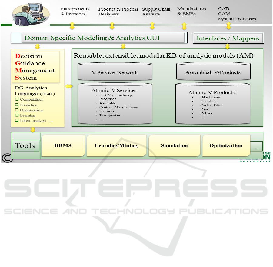
Figure 1: SPOT architecture based on DGMS.

4 ANALYTIC PERFORMANCE

MODEL FOR PARAMETERED

PRODUCTS AND SERVICES

4.1 Parameterized Optimization

Problem

Optimization models for VSPs are predicated on the

notion of an analytic performance model (AM). Intu-

itively, AM describes the output of performance met-

rics (such as weight and cost) and feasibility con-

straints as a function of input. This input consists

of ﬁxed decision parameters such as product proper-

ties, quantities of products purchased, and settings of

manufacturing processes. More formally, an AM is a

function:

AM : I → O (1)

where I and O are valid input and output domains.

The function AM yields the output AM(i) ∈ O for i ∈ I

which captures customer-facing metrics.

To ﬁnd optimal values of decision parameters in

the input, we can choose an objective function that

gives a real value for every output o ∈ O

Ob j : O → R

as well as constraint

C : O → {T, F}

that yields a Boolean value for every output o ∈ O

to indicate whether it is feasible (C(o) = T ) or not

(C(o) = F).

We are interested in solving optimization prob-

lems of the form

min\max

x∈I

Ob j(AM(x))

s.t. C(AM(x))

(2)

Note that, while the objective and the constraints in

the optimization problems are expressed in terms of

input i ∈ I, our formulation based on AMs allows ﬂex-

ible expression of a range of optimization problems,

with no need to modify the AM, which “hides” a pos-

sibly involved code that expresses its function. For-

malizing the objective function and constraints in this

manner leads to a natural decomposition of the prob-

lem statement into separate categories that intuitively

reﬂect the product and process speciﬁcations.

In the remainder of Section 4 we describe the AM

for a (hierarchically) composed service network with

ﬂexible products, using the example of a bicycle man-

ufacturing supply chain. To do this, we ﬁrst describe

the structure of a valid output from the AM in Sec-

tion 4.2, then a valid input in the AM in Section 4.3,

and, ﬁnally, the computation ﬂow of the AM, in Sec-

tion 4.4, which maps a valid input instance to a valid

output.

SPOT: Toward a Decision Guidance System for Uniﬁed Product and Service Network Design

721

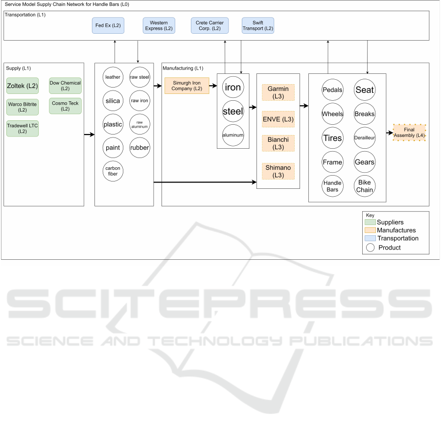
Figure 2: Supply Chain Product and Service Flow.

In the following, we use the following notation of a

set of key-value pairs of the form:

{key

: value

, . . . , key

: value

}

where the keys are unique identiﬁers. Note, that

this structure represents a mapping m from the set of

keys {key

, . . . , key

} to the union ∪

i=1

of domains

, i = 1, ..., k, such that m(key

) ∈ D

. Thus m(key

)

represents value

, i = 1, . . . , n.

4.2 Model Output Structure

An output o of the analytic model represent metrics

of interest and constraints in the form of a set of key :

value pairs:

{ metric

: value

... ,

metric

: value

constraints: True or False

rootService: root service id

services: <set of services>

products: <set of products> }

(3)

as follows.

Metrics 1. through n are additive metrics of the root

service (see below) such as the total cost and carbon

emissions. Note that these metrics are not ﬁxed as

they are aggregated, recursively, from atomic services

up.

Constraints: are True, if all the feasibility constraints

of the service network under the root service and the

products associated with it, as described under ser-

vices, are satisﬁed.

rootService: is the id of the root service, to distin-

guish it from the other services, which are described

next.

Services: is a set of key-value pairs of the form:

{ sid

: service

... ,

sid

: service

}

(4)

where the sids are unique service identiﬁers, includ-

ing the root service. Each service 1 through n is ei-

ther composite or atomic. Composite services have

sub-services, whereas atomic services do not. Each

composite service output is a set of key-value pairs of

the form:

{ type: “composite”

metric

: value

... ,

metric

: value

constrains: True or False

inFlow: ﬂows of consumed products

outFlow: ﬂows of produced products

subServices: set of sub-service ids }

(5)

ICEIS 2021 - 23rd International Conference on Enterprise Information Systems

722

type indicates the type of the service, and is “com-

posite” here for the composite service.

metrics 1 through n are the same as the metrics in

equation (3). Each metric is additive, i.e., it is the sum

of the values for this metric across all (child) subSer-

vices, described below.

constraints is the conjunction of sub-service con-

straints, and the ﬂow balancing constraints within the

service. These are described formally in Section 4.4.

inFlow and outFlow describe the ﬂows of con-

sumed and produced products, respectively. Each is

of the following form:

{ f id

:{ qty: real number

item: pid},

... ,

f id

:{ qty: real number

item: pid}

(6)

where ﬁds are unique ﬂow identiﬁers, where corre-

sponding qty is the quantity (being consumed or pro-

duced), and pid is the unique identiﬁer of a product

associated with the ﬂow. subServices is a set of ids of

sub-services of this composite service.

Each atomic service is the same form as equation

(5) for composite service with a few exceptions. First,

the object subService is not present because atomic

services do not have sub-services. Second, type

maybe any string not logically equivalent to “com-

posite”. In our example in Section 2, we use the string

“supplier” and “transport” to distinguish atomic ser-

vices from each other. Third, the metrics, constraints,

inFlows, and outFlows are speciﬁc to the atomic ser-

vice. Thus, each atomic service output is a set of key-

value pairs of the form:

{ type: !=“composite”

metric

: value

... ,

metric

: value

constrains: True or False

inFlow: ﬂows of consumed products

outFlow: ﬂows of produced products }

(7)

Products: is a set of key-value pairs of the form:

{ pid

: product

... ,

pid

: product

}

(8)

where pid are ids of the products. Each product 1

through n is of the form

{ type: basic or assembled}

metric

: value

...,

metric

: value

constraint : True or False }

(9)

where type is either an basic or assembled prod-

uct. Assembled products are constructed from other

products within the supply network and are labeled

assembled under type. Products also contains a se-

ries of constrains. These constraints specify thresh-

olds or acceptable materials for use. Our products

object is then given to us by the following n-tuple:

4.3 Model Input Structure

A valid VP input instance i is a set of key-value pairs

{ shared: <general-shared-info>

ﬂows: <set of ﬂow ids>

rootService: root service id

services: <set of services>

products: <set of products> }

(10)

Shared: contains all data required for computation

in multiple layers of security or computation. For ex-

ample, the location of each manufacturer is required

in the computation of transportation services (see

Section 2) and it is also required in the optimization

of environmental metrics for material selection (see

Section 2). The structure of Shared is:

{ shared

: {real-value, text},

... ,

shared

: {real-value, text} }

(11)

Flows: contains a list of ﬂow ids for all ﬂows within

the supply network. Each ﬂow id has one child which

is the product id. Within any supply network there

can be n such ﬂows. Thus, we deﬁne our ﬂow object

as,

{ f id

: pid

f id

: pid

... ,

f id

: pid

}

(12)

rootService: is the id of the root service being evalu-

ated. It is deﬁned the same as in equation (3).

Services: are deﬁned as follows for composite and

atomic services:

{ type: ‘composite’

inFlow: <set of inﬂow ids>

outFlow: <set of ﬂow ids>

subServices: <set of sub-service ids> }

(13)

{ type: ‘atomic’

inFlow: <set of inﬂow ids>

outFlow: <set of ﬂow ids>

ppu info: <set of model pricing data>

qtyInPer1Out: <set of ﬂow ids> }

(14)

type indicates if a service is a composite or non-

composite.

SPOT: Toward a Decision Guidance System for Uniﬁed Product and Service Network Design

723

inFlow and outFlow are lists of unique ids indi-

cating which products were consumed and produced

during manufacturing. An illustration of the supply

ﬂows is illustrated in Section 2. In addition, each el-

ement holds a feature labeled lb and units. lb is a

real-valued number giving our low bound on the ﬂow.

units refers to the units the quantity is measured in.

subServices are deﬁned the same way as in equa-

tion (5) and only appear in composite services.

ppu info is an n-tuple object with n different prod-

ucts being product by the service. For each prod-

uct produced, a 2-tuple object containing the type of

model that should be used for calculating the price per

unit and the pricing model’s features. These features

correspond to each of the products’ properties listed

in the products object. ppu in f o is only present for

atomic services.

qtyInPer1Out is an n-tuple object with n different

products being produced by the service. For each

product produced, a product and quantity is listed

which indicates the amount required to product one

unit of output. This object is only present in services

with the type manufacturer.

orders is an n-tuple object with n different

products being transported by the service. For each

product transported, the following data structure is

present:

{ in: ﬁd

out: ﬁd

sender: sid

recipient: sid

qty: {real value} }

(15)

where in is the ﬂow id of the incoming product to

be transported, out is the ﬂow ids after the product

has been transported, sender is the service id of the

sender, recipient is the service id of the recipient of

the product, and qty is the amount of product within

the shipment.

Products: are deﬁned as follows. Each product p

in the set P is labeled as either a basic or assembled

product. Assembled products are constructed from

other products within the supply network and are la-

beled assembled under type. Assembled products are

also given an additional feature that basic products do

not have; components.

Components are lists of product names that are

used as input material. Each element in this object

contains a value x ∈ N which indicates the quantity of

that component required for assembly.

Constraints are restrictions on the physical prop-

erties of the product. This can either be a real-valued

tolerance level of a physical property (like weight

or height) or a limitation on the types of materials

the product is made out of (like aluminum or carbon

ﬁber).

In addition, products has an entry for each physi-

cal property pertinent for analysis. Our products ob-

ject is deﬁned by the following n-tuple:

{ type: basic or assembled

components: list

constraint

: {real-value, list}

constraint

: {real-value, list}

property

: {real-value, text} }

(16)

4.4 Analytic Model: Computing Output

from Input

In this Section we describe the computation of the

valid output from a valid input. We describe the

computation top-down, recursively, starting with the

overall service network analytic model, followed by

the composite service, atomic services, composite

(assembled) product model, and ﬁnally the atomic

product models.

Model Output. The output o of the AM, described

in (3) is computed from the input i, described in (10),

as follows. Let services = o(services), products =

o(products) deﬁned later in this section. Let rootid =

i(rootService) and productIds = keys(i(products)).

Then the values for each metric m

, i = 1, ..., n, in the

output o is taken from the root service:

o(m

) = services(rootid)(m

)

The constraints are given by

constrains = services(rootid)(constraints) ∧

productConstraints

where productConstraints =

∀sp ∈ productIds :

products(sp)(constraints)

Computation of Composite Service. Here we de-

scribe the computation of valid output for a compos-

ite service in equation (5). Let s be an id of a service

in services in equation (4). Then, services(s) is a set

of key-value pairs in equation (5). The value for key

type is services(s)(type) = “composite”. The value

services(s)(m

) for each metric m

, i = 1, ..., n is given

by:

services(s)(m

) =

∑

ss∈SS

service(ss)(m

)

where SS = services(s)(subServices) is the set of sub-

service ids.

ICEIS 2021 - 23rd International Conference on Enterprise Information Systems

724

To describe the computation of inFlow, outFlow,

and constrains for service s, we ﬁrst deﬁne a number

of concepts.

Let

serviceFlows =

keys(services(s)(inFlow)) ∪

keys(services(s)(outFlow))

(17)

subServiceFlows =

∪

ss∈SS

keys(services(ss)(inFlow)) ∪

∪

ss∈SS

keys(services(ss)(outFlow))

(18)

allFlows =

serviceFlows ∪ subServicesFlows

(19)

internalFlows =

subServicesFlows − serviceFlows

(20)

be the service ﬂows, the sub-services’ ﬂows, all ﬂows,

and the internal only ﬂows respectively. For every

ﬂow f ∈ allFlows, we deﬁne the internal supply of

ﬂow f as:

internalSupply( f ) =

∑

ss∈SS

outQty(ss, f )

(21)

where

outQty(ss, f ) = service(ss)(outFlow)( f )(qty) (22)

if f ∈ keys(service(ss)(outFlow)), and 0 otherwise.

Similarly, internalDemand( f ) is computed by re-

placing the key “outFlow” with the key “inFlow” in

equation (21).

The following is the balancing constraint for ﬂow

supply and demand, as follows:

internalSupplySatis f iesDemands =

∀ f ∈ internalFlows :

internalSupply( f ) ≥ internalDemand( f )

(23)

Let inFlowIds = keys(i(services)(s)(inFlow)) and

outFlowIds = keys(i(services)(s)(outFlow)) be the

inFlow and outFlow ids of service s. We deﬁne

inFlow = o(services)(s)(inFlow) by

∀ f ∈ inFlowsIds :

inFlow( f ) =

internalDemand( f ) − internalSupply( f )

(24)

Similarly, outFlow = o(services)(s)(outFlow) is de-

ﬁned by

∀ f ∈ outFlowsIds :

outFlow( f ) =

internalDemand( f ) − internalSupply( f )

(25)

The inFlowConstraints and outFlowConstraints are

bound constraints given by

inFlowConstraints =

f lowBoundConstraints(inFlow

, inFlow)

(26)

outFlowConstraints =

f lowBoundConstraints(outFlow

, outFlow)

(27)

where inFlow

= i(services)(s)(inFlow) and

outFlow

= i(services)(s)(outFlow), respec-

tively taken from the input i. The predicate

f lowBoundConstraints( f lowBounds, f low) is given

∀ f ∈ f lows :

f lows( f )(qty) ≥ 0 ∧

f lows( f )(qty) ≥ f lowBounds( f )(lb)

(28)

We deﬁne subServiceConstraints recursively as

subServiceConstraints =

∀ss ∈ services(s)(subServices) :

services(ss)(constraints)

(29)

We now deﬁne the overall constraints is the conjunc-

tion:

constraints =

internalSupplySatis f iesDemand ∧

inFlowConstraints ∧

outFlowConstraints ∧

subServiceConstraints

(30)

Finally, deﬁne subService to be a copy of the

subService structure deﬁned in (13).

Computation of Atomic Services. For every atomic

service with id s, a valid output services(s) is of

the form described in Structure (7). The extensible

library of atomic services initially includes models

for suppliers, manufacturers and transportation as

follows.

Suppliers: The type services(s)(type) = “Supplier”.

The cost services(s)(cost) is computed as

∑

o∈outFlows

computePPU(products, ppu

in f o)∗

outﬂow(o)(qty)

(31)

where products and ppu in f o are

equal to products( f lows(o)) and

ppu in f o( f lows(o))(product ppu), f lows and

products are from the input Structure (10). The

function computePPU is a function which produces

the price-per-unit of a product as determined by the

business operational parameters deﬁned in ppu in f o,

the products physical properties deﬁned in equation

(9), and the products required performance thresholds

SPOT: Toward a Decision Guidance System for Uniﬁed Product and Service Network Design

725

also deﬁned in equation (9).

We now deﬁne the value for inFlow and outFlow.

For our Supplier type atomic service, it is assumed

that the supplier does not require any products from

any other service to produce output. Services that do

require input from other services within the supply

chain are deﬁned as Manu f actures.

The inﬂow services(s)(inFlow) is deﬁned as the

empty set of key-value pairs:

inFlow(qty) = {}

(32)

Let outFlow

= i(services)(s)(outFlow) where i

is the input and f lows = i( f lows) as deﬁned as

in the data structure (10). Then, the outﬂow

services(s)(outFlow) is deﬁned as follows:

∀o ∈ keys(outFlow

)

outFlow(o)(qty) = outFlow

(o)(qty)

outFlow(o)(item) = f lows(o)

(33)

We now deﬁne constrains for a valid supplier atomic

service output.

constraints =

inFlowConstraints ∧

outFlowConstraints

(34)

The inFlowConstraint and outFlowConstraint val-

ues are deﬁned as:

f lowBoundConstraints(inFlow

, InFlow) (35)

f lowBoundConstraints(outFlow

, OutFlow) (36)

where the function f lowBoundConstraints is as

deﬁned as before in equation (28), inFlow

and

outFlow

are deﬁned in the same fashion as equation

(26) and (27).

Manufactures: The type services(s)(type) =

“Manu f acturer.” The value for cost

services(s)(cost), outﬂow services(s)(outFlow),

and constraints services(s)(constrains) are com-

puted as described in equations (31), (33), and (34)

respectively.

To compute inFlow, let qtyInPer1out

be i(services)(s)(qtyInPer1out), out f low

be services(s)(outFlow), and inFlow

i(services)(s)(inFlow) where i is the input de-

scribed in data structure (14).

Then, the inﬂow services(s)(inFlow) is computed as

follows:

∀ f ∈ keys(inFlow

) :

services(s)(inFlow)( f ) =

qtyInPer1out( f ) ∗ out f low( f )(qty)

(37)

Transportation: The type services(s)(type) =

“Transportation.”

Let inFlow

, outFlow

, orders and f lows be

i(services)(s)(inFlow), i(services)(s)(outFlow),

i(services)(s)(orders) and i( f lows) respectively,

where i is the input described in Structure 10. Then,

the inﬂow services(s)(inFlow) is deﬁned as follows:

∀ f ∈ inFlow

inFlow( f )(qty) =

∑

o∈relevantOrders( f )

o(qty)

inFlow( f )(item) = f lows( f )

(38)

where inFlow = services(s)(inFlow) and

relevantOrders( f ) = {o ∈ orders | o(in) = f }.

Similarly, outFlow services(s)(outFlow) is deﬁned

as follows:

∀ f ∈ out f low

outFlow( f )(qty) =

∑

o∈relevantOrders( f )

o(qty)

outFlow( f )(item) = f lows( f )

(39)

where outFlow = services(s)(outFlow) and

relevantOrders( f ) = {o ∈ orders | o(out) = f }.

The value for constrains is deﬁned in equation

(34) with the ﬂow objects deﬁned in the equations

listed above for in f low and out f low.

Computation of Assembled Products. Here we

describe the computation of valid output for a as-

sembled product in equation (9). Let p be an id of a

product deﬁned in equation (16). The, products(p) is

a set of key-value pairs in equation (9). The value for

key type is products(p)(type) = “assembled”. The

value products(p)(m

) for each metric m

, i = 1, ...,n

is given by:

products(p)(m

) =

∑

c∈C

products(c)(m

)

where C = products(p)(components) is the set of

product ids.

Let m

be a metric calculated in equation (9) for

product p. Let lb and ub be the lower-bound and

upper-bound for metric m

. We deﬁne the value for

constraints

in the following way:

products(p)(lb) ≤ m

≤ products(p)(ub)

where product is from the input data structure

deﬁned in equation (16).

Computation of Basic Products. The output re-

turned for the computation of basic products is copy

of the input described in equation (14).

ICEIS 2021 - 23rd International Conference on Enterprise Information Systems

726

5 SPOT METHODOLOGY BY

EXAMPLE

In this Section, we demonstrate how a user can use

SPOT to optimize over products and services to gen-

erate the supply chain for a Virtual Bicycle described

in Section 2. The demonstration is organized as fol-

lows: (1) a general description of valid input construc-

tion, (2) selection of a valid solver, (3) submitting the

valid input to SPOT, (4) interpreting the results.

The ﬁrst task to be completed is the construction

of a valid input JSON ﬁle. Requirements for this task

include a JSON editor, domain knowledge of supply

chain network (e.g. Figure ??) or access to a stored

repository which contains the structure of the supply

chain network, knowledge of manufactures pricing

models or access to the stored repository of manufac-

turers pricing, and miscellaneous documents required

to create a valid input data structure described in Sec-

tion 4.3.

The user will create a JSON object similarly to

the one deﬁned in the Data Structure (10). Using a

graphic similar to Figure (2), a hierarchical relation-

ship between the different service levels should be

created. A the top level (e.g. L0), the rootService

should be given a name that is demonstrative of

the supply chain’s purpose. For our example our

rootService is given the value “bikeSupplyChain”.

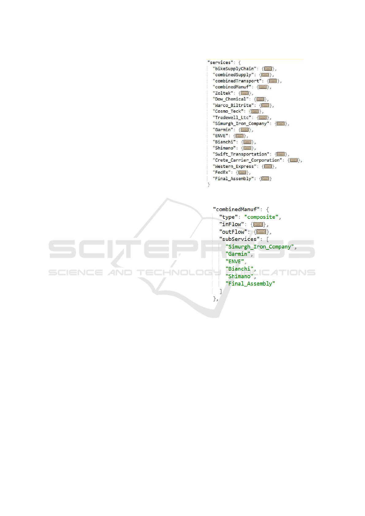
Next, the user will populate the composite service

“bikeSupplyChain” in the object services. This is

done because SPOT views the top-level domain as a

composite service. Thus, the type for “bikeSupply-

Chain” is equal to “composite”. The object inFlow

should be an empty object because each of our initial

services is a supplier. The outFlow object contains

our end product ﬁd (e.g. bike01). Our subService ob-

ject contain the sids of the service that comprise of the

bikeSupplyChain. In our case, we have three services:

combinedSupply, combinedManufacturing, and com-

binedTransportation.

The next level in our services model is L1 which

comprise of each of the composite service which

make up bikeSupplyChain. For each composite ser-

vice the user should populate the JSON object with

the Structure deﬁned in Data Structure (13) making

special care to ﬁll in the subServices object with the

desired hierarchical service network model as illus-

trated in Figure (4). Using a graphic similar to Fig-

ure (??) each service’s ﬂow object should be popu-

lated with the correct ﬂows described in Data Struc-

ture (12). This process continues for until each com-

posite and atomic service has been added to the ser-

vice object described in Section (4.3).

Figure 3: Valid Service Input Data Structure.

Figure 4: Valid Sub-Service Input Data Structure.

Next, we must analyze our objective function in

relation to the constraints and identify if we should

use a linear or non-linear solver. The beneﬁts of using

a linear solver over a non-linear solver is improved

running time. In our case, we ﬁnd that our objective

function is a linear programming problem.

We submit the input data to SPOT by specifying

the model, input data, objective function, constraints,

the problem type, the solver, and debug ﬂag. The an-

swer to the optimization problem is reported back as

a JSON ﬁle as described in Section (4.2).

The output in Figure (5) is a valid output data

structure from SPOT. The metrics for the optimal se-

lection of services and products are displayed at each

of level of the hierarchical supply chain network. Fig-

ure (5) displays the top-level metrics. In addition,

the Boolean value of the constraints are displayed.

Traversing the output down service will reveal each

SPOT: Toward a Decision Guidance System for Uniﬁed Product and Service Network Design

727

Figure 5: Valid Output Data Structure.

of the metrics for the Sub-Service which comprise of

the bikeSupplyChain.

6 CONCLUSION AND FUTURE

RESEARCH

This research is the ﬁrst step toward developing a

decision guidance system for combined optimization

over product design, process design, and supply chain

management all while keeping the lower level math-

ematical programming code hidden from the domain

users. The prototype, SPOT, was successfully tested

on a virtual bicycle product and service network.

The methodology in creating hierarchical data input,

which describes the assembly of product and services

using the described input data structure, successfully

generated a valid output data structure with the cor-

rect optimal solution. This modular composite of the

life cycle of product design is unique in the fact that

it joins the optimization of traditionally silo’d project

spaces and adds to the agility of realizing product

and services using distributed manufacturing capac-

ity. Many research questions remain open. Future

research directions include expanding the functional-

ity of SPOT, integrating the application with existing

design tools such as CAD and CAM, creating a graph-

ical user interface to design the hierarchical relation-

ships.

REFERENCES

Towards agile engineering of mechatronic systems in ma-

chinery and plant construction.

Brodsky, A., Gingold, Y., LaToza, T. D., Yu, L.-F., and Han,

X. (2021). Catalyzing the agility, accessibility, and

predictability of the manufacturing-entrepreneurship

ecosystem through design environments and markets

for virtual things. In 10th Intern. Conf. on Oper-

ations Research and Enterprise Systems (ICORES-

2021), pages 264–272.

Brodsky, A., Krishnamoorthy, M., Bernstein, W. Z., and

Nachawati, M. O. (2016). A system and architecture

for reusable abstractions of manufacturing processes.

In 2016 IEEE International Conference on Big Data

(Big Data), pages 2004–2013.

Brodsky, A., Krishnamoorthy, M., Nachawati, M. O., Bern-

stein, W. Z., and Menasc

e, D. A. (2017). Manufactur-

ing and contract service networks: Composition, op-

timization and tradeoff analysis based on a reusable

repository of performance models. In 2017 IEEE In-

ternational Conference on Big Data (Big Data), pages

1716–1725.

Brodsky, A., Nachawati, M. O., Krishnamoorthy, M., Bern-

stein, W. Z., and Menasc

e, D. A. (2019). Factory op-

tima: a web-based system for composition and anal-

ysis of manufacturing service networks based on a

reusable model repository. International Journal of

Computer Integrated Manufacturing, 32(3):206–224.

Denkena, B., Shpitalni, M., Kowalski, P., Molcho, G., and

Zipori, Y. (2007). Knowledge management in process

planning. CIRP Annals, 56(1):175 – 180.

Eddy, D. C., Krishnamurty, S., Grosse, I. R., Wileden, J. C.,

and Lewis, K. E. (2015). A predictive modelling-

based material selection method for sustainable prod-

uct design. Journal of Engineering Design, 26(10-

12):365–390.

Garcia, D. J. and You, F. (2015). Supply chain design and

optimization: Challenges and opportunities. Comput-

ers & Chemical Engineering, 81:153 – 170. Special

Issue: Selected papers from the 8th International Sym-

posium on the Foundations of Computer-Aided Pro-

cess Design (FOCAPD 2014), July 13-17, 2014, Cle

Elum, Washington, USA.

Helu, M. and Hedberg, T. (2015). Enabling smart manufac-

turing research and development using a product life-

cycle test bed. Procedia Manufacturing, 1:86 – 97.

43rd North American Manufacturing Research Con-

ference, NAMRC 43, 8-12 June 2015, UNC Charlotte,

North Carolina, United States.

Herrmann, J., Cooper, J., Gupta, S., Hayes, C., Ishii, K.,

Kazmer, D., Sandborn, P., and Wood, W. (2004). New

directions in design for manufacturing. volume 3.

Klingstam, P. and Gullander, P. (1999). Overview of simula-

tion tools for computer-aided production engineering.

Computers in Industry, 38(2):173 – 186.

McLean, C. and Shao, G. (2003). Manufacturing case stud-

ies: Generic case studies for manufacturing simula-

tion applications. In Proceedings of the 35th Confer-

ence on Winter Simulation: Driving Innovation, WSC

’03, page 1217–1224. Winter Simulation Conference.

Molcho, G., Zipori, Y., Schneor, R., Rosen, O., Goldstein,

D., and Shpitalni, M. (2008). Computer aided manu-

facturability analysis: Closing the knowledge gap be-

tween the designer and the manufacturer. CIRP An-

nals, 57(1):153 – 158.

Salvendy, G. (2001). Handbook of Industrial Engineering:

Technology and Operations Management.

Shehadi, A. I.-H. S. (2019). On the move: manufacturing’s

return to the developed world. FDiIntelligence.

Stoll, H. W. (1986). Design for Manufacture: An Overview.

Applied Mechanics Reviews, 39(9):1356–1364.

Wu, D., Greer, M. J., Rosen, D. W., and Schaefer, D. (2013).

Cloud manufacturing: Strategic vision and state-of-

the-art. Journal of Manufacturing Systems, 32(4):564

– 579.

ICEIS 2021 - 23rd International Conference on Enterprise Information Systems

728