Comparison of Camera-Equipped Drones and Infrastructure Sensors for

Creating Trajectory Datasets of Road Users

Amarin Kloeker

, Robert Krajewski

and Lutz Eckstein

Institute for Automotive Engineering, RWTH Aachen University, Steinbachstr. 7, 52074 Aachen, Germany

Keywords:

Automated Driving, Trajectory Dataset, Drone, Infrastructure Sensors, ITS-S, Computer Vision.

Abstract:

Due to the complexity of automated vehicles, their development and validation require large amounts of nat-

uralistic trajectory data of road users. In addition to the classical approach of using measurement vehicles

to generate these data, approaches based on infrastructure sensors and drones have become increasingly pop-

ular. While advantages are postulated for each method, a practical comparison of the methods based on

measurements of real trafﬁc has so far been lacking. We present a theoretical and experimental analysis of two

image-based measurement methods. For this purpose, we compare measurements of a drone-based system

with a prototypical camera-based infrastructure sensor system. In addition to the detection statistics of the

road users, the detection quality of both systems is also investigated using a reference vehicle equipped with

an inertial navigation system. Through these experiments, we can conﬁrm each approach’s advantages and

disadvantages emerging from the theoretical analysis.

1 INTRODUCTION

The development of automated vehicles is a trend that

will signiﬁcantly shape the trafﬁc of the future. In-

telligent systems will gradually take over the driving

task from the driver, thereby increasing the safety,

comfort and efﬁciency of future mobility. On the

way to fully automated driving, however, a number

of challenges have to be overcome. In comparison

to a simple advanced driver assistance system, an au-

tomated vehicle has a large number of sensors such

as cameras, radars and LiDARs. Through these sen-

sors, it must perceive its immediate static as well as

dynamic environment precisely. Furthermore, an au-

tomated system has to take over the control of the ve-

hicle permanently instead of only rarely being really

active, like e.g. an emergency braking system. Fi-

nally, the Operational Design Domain or the number

of possible scenarios is large, especially in urban ar-

eas.

Due to the resulting complexity, many problems

during the development and validation of automated

vehicles are no longer solved conventionally, but data-

driven. This development started with perception, for

which camera images have been processed by neu-

https://orcid.org/0000-0003-4984-2797

https://orcid.org/0000-0001-7288-0172

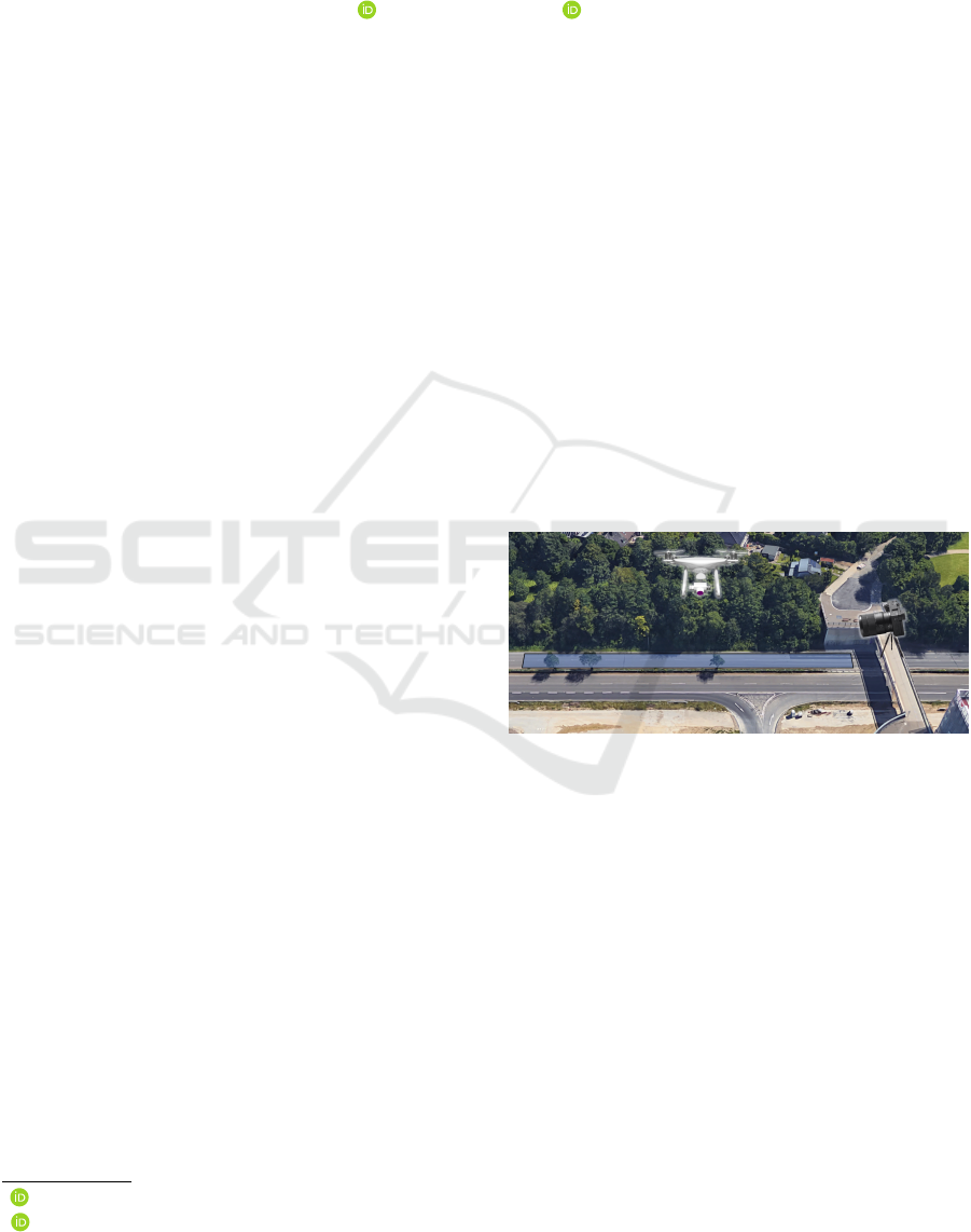
Figure 1: Visualization of the measurement setup. A drone-

based measurement system is compared to a camera-based

system positioned on a bridge. The blue box indicates the

recorded area.

ral networks for years in research in order to solve

issues such as the detection of other road users. In

the meantime, however, other components of an auto-

mated driving system, such as the modeling and pre-

diction of road user behavior, have also become data-

driven. This is necessary for an automated vehicle

to calculate a safe trajectory. Lastly, it has already

been shown that even for simple highway systems the

number of possible driving scenarios cannot be tested

conventionally. This would require more than 1.3 bil-

lion test kilometers (Winner et al., 2015). Instead, in-

telligent, scenario-based testing becomes necessary.

For the extraction, modeling and statistical analysis

of these scenarios, trajectory data are absolutely nec-

essary.

Kloeker, A., Krajewski, R. and Eckstein, L.

Comparison of Camera-Equipped Drones and Infrastructure Sensors for Creating Trajectory Datasets of Road Users.

DOI: 10.5220/0010458001610170

In Proceedings of the 7th International Conference on Vehicle Technology and Intelligent Transport Systems (VEHITS 2021), pages 161-170

ISBN: 978-989-758-513-5

161

Most publicly accessible datasets available today

are devoted to perception tasks in line with the devel-

opment in the use of data-driven methods. Among

the best-known examples are KITTI (Geiger et al.,

2013) and Cityscapes (Cordts et al., 2016), which

contain annotated camera and LiDAR data. In com-

parison, trajectory datasets with a focus on automated

driving have typically appeared later and are smaller

(e.g. (Robicquet et al., 2016)). This is partly due

to the slower penetration of data-driven methods for

e.g. prediction tasks. On the other hand, the cre-

ation of trajectory datasets is usually much more com-

plex. While for perception datasets typically only sin-

gle frames or short sequences are annotated manu-

ally or semi-automatically, which is already very la-

borious, for trajectory datasets a continuous annota-

tion of all frames is essential to preserve the temporal

dimension. Since this is not possible in a meaning-

ful way manually, fully automated processing systems

are necessary.

While sensor datasets for automated driving must

almost inevitably be recorded with a vehicle-bound

sensor system, there are more possibilities when de-

signing a measuring system for trajectory data. Be-

sides the use of measurement vehicles, infrastruc-

ture sensors and drones are established alternatives.

While measurement vehicles often fuse different sen-

sor types, so far systems based on drones (e.g. (Kra-

jewski et al., 2018)) and infrastructure sensors (Col-

yar and Halkias, 2007) mainly work with cameras.

Only recently have LiDAR sensors become more ad-

vanced and more affordable, so that they are also used

in current systems (Kloeker et al., 2020). The choice

of the sensor-bearing system and the selection of the

sensors used are subject to individual advantages and

disadvantages (Krajewski et al., 2018). It is plausi-

ble, for example, that an elevated recording position

of the sensors reduces vehicle-to-vehicle occlusions.

However, a theoretical and experimental investigation

of the resulting consequences for trajectory datasets

is missing so far. Furthermore, a practical compari-

son of several methods with each other based on real

measured data in a typical recording scenario is ab-

sent.

In this publication, we would like to contribute to

closing this gap. We compare two popular approaches

to the generation of trajectory datasets. We investigate

theoretically and experimentally assumed or postu-

lated (dis-)advantages. Further, we evaluate their ac-

tual relevance for the generation of trajectory datasets.

Our main contributions are:

• We develop a prototypical camera-based measure-

ment system to generate trajectory datasets from

trafﬁc recordings taken by a camera positioned on

a bridge

• We theoretically analyze the advantages and lim-

itations of this system compared to a drone-based

system

• We experimentally compare both systems with re-

spect to the detection statistics of non-instructed

passing trafﬁc and a reference vehicle equipped

with a highly accurate inertial navigation system

(INS)

2 RELATED WORK

With the increasing need for datasets due to the grow-

ing popularity of data-driven approaches in the ﬁeld

of automated driving, the number of approaches to

create them is growing as well. The development

started with the creation of sensor datasets for per-

ception problems, in which e.g. all dynamic road

users are annotated by bounding boxes or the static in-

frastructure is semantically segmented. Well-known

representatives are the KITTI dataset (Geiger et al.,

2013) and the Cityscapes dataset (Cordts et al., 2016).

The relevance of these datasets is not only shown by

the number of citations, but also by the competing

datasets published in the following years. However,

since usually only single points in time or very short

sequences of frames are annotated, the necessary tem-

poral context is missing, which is required e.g. for

prediction problems. An exception to these datasets

from the vehicle perspective is the Level 5 dataset

(Houston et al., 2020), which was developed espe-

cially for prediction tasks, and the Five Roundabouts

dataset (Zyner et al., 2019). However, these datasets

do not consist of manual annotations, but of auto-

mated detections based on a sensor fusion of camera

and LiDAR data or only LiDAR data. Due to the per-

spective and occlusions, signiﬁcant errors are present

in the detections, so that the prediction task cannot be

considered separately from the characteristics of the

used sensor technology.

More common are therefore approaches based on

the use of permanently installed infrastructure sensors

and drones hovering above the trafﬁc. The ﬁrst dataset

published from the drone perspective is the Stanford

Drone Dataset (Robicquet et al., 2016), which fo-

cuses on trafﬁc participants on a university campus.

While this dataset is still based on classical tracking

approaches, the datasets published later use a more

complex processing pipeline. For the creation of

the highD dataset (Krajewski et al., 2018) the video

recordings were stabilized, all road users were de-

VEHITS 2021 - 7th International Conference on Vehicle Technology and Intelligent Transport Systems

162

tected by neural networks, and trajectories were ex-

tracted by a tracking algorithm and RTS smoother

(Rauch et al., 1965). Other datasets like the inD

dataset (Bock et al., 2020), rounD dataset (Krajew-

ski et al., 2020), INTERACTION dataset (Zhan et al.,

2019) or TOPVIEW dataset (Yang et al., 2019) all use

a very similar pipeline, but focus on different trafﬁc

scenarios. In (Kruber et al., 2020) the measurement

accuracy of drone-based systems is investigated using

a reference vehicle equipped with an inertial naviga-

tion system.

In addition to the ability to ﬂy dynamically at var-

ious locations and to detect the behavior of road users

unnoticeably, the drone has a distinct advantage over

other approaches. Due to the bird’s eye view, there

are almost no vehicle-vehicle occlusions if the drone

is correctly positioned so that a global image of the

trafﬁc is obtained. Further, the vehicles have to be

tracked in 2D only. In order to exploit this potential,

however, a high-resolution camera, precise video sta-

bilization and deep-learning-based tracking systems

are required.

Infrastructure sensors are usually used in the form

of an intelligent transportation system station (ITS-

S). Typically an elevated positioning is used for the

sensors to gain perspective advantages. The percep-

tion of existing datasets consists mostly of single or

fused cameras. While for some datasets single cam-

eras were used, the fusion of several cameras allows

to observe a greater area. For the NGSIM (Colyar

and Halkias, 2007) and Ko-PER (Strigel et al., 2014)

datasets, cameras were positioned on infrastructure

elements, like buildings and lamp posts, to observe

a highway section or a full intersection. Similar to

the development of algorithms for processing drone

images, these older systems are based on more clas-

sical approaches and work on lower-resolution cam-

era images. In contrast, current approaches such as

the INTERACTION dataset (Zhan et al., 2019) use

high-resolution cameras and neural networks to pre-

cisely detect road users. At the same time, there are

also research projects that cover intersections or large

sections of highways on a camera-based basis but do

not provide data (AIM (Schnieder et al., 2013), Test

Field Lower Saxony (K

oster et al., 2018)). Recently

it has also become feasible to additionally equip the

ITS-Ss with highly accurate LiDAR sensors to further

improve the detection accuracy (Kloeker et al., 2020).

The main advantage of ITS-Ss is their high efﬁ-

ciency, once they are installed. Unlike a drone, which

in the best case can only record up to one hour at a

time, ITS-Ss theoretically allow unlimited recording

times. However, this is at the expense of the lack

of ﬂexibility. A disadvantage associated with ITS-Ss

compared to a drone is the perspective causing occlu-

sions and degrading tracking accuracy with increas-

ing distance from the sensors. To handle these prob-

lems, in most cases, multiple types of sensors also po-

sitioned at different locations are combined (Kloeker

et al., 2020; Kr

ammer et al., 2019).

So far, there exists no comparison between drones

and stationary camera sensors on real, synchronous

measurements. For the INTERACTION dataset, a

simulative quality evaluation was performed for a sta-

tionary camera, but no real tests (Zhan et al., 2019).

The DLRAD dataset (Kurz et al., 2018) provides data

from an aerial perspective recorded with a helicopter

but neither an evaluation nor the dataset is released.

Within the Providentia test site, reference measure-

ments were also generated with a helicopter, but were

considered as ground truth for evaluating the infras-

tructure (Kr

ammer et al., 2019). No comparison was

made between the two approaches.

3 METHOD

We propose a comparison of both fundamental ap-

proaches under optimal conditions. These include the

weather, lighting, visibility and infrastructure-caused

occlusions. For the comparison, we perform joint

recordings with a drone-based system as well as with

a prototypical single-camera-sensor-based ITS-S (see

Fig. 1). While we use exactly the drone and process-

ing system also used for the creation of the highD

dataset (Krajewski et al., 2018) for the processing of

the videos from the bird’s eye view, we create a sepa-

rate system for the processing of infrastructure-based

recordings. Both approaches can theoretically be ex-

tended without limitations by using any number of

drones or sensors. For a fair comparison, we use only

a single sensor for each system and try to create as

equal conditions as possible. Both systems use a sin-

gle high-resolution 4K camera that records trafﬁc at

25 FPS. Further, the hardware costs and effort dur-

ing the recording process are comparable. As a result,

we get a fundamental comparison of the two perspec-

tives.

For a comprehensive comparison, we suggest

three steps, one of which is theoretical while the other

two are experimental. In the ﬁrst step, an analy-

sis of the presented systems will be used to derive

the theoretically achievable quality and limitations of

both approaches, taking into account the individual

components. The other two steps verify these ﬁnd-

ings by practical experiments. In the second step,

the detection statistics of random trafﬁc in the con-

sidered road section will be evaluated. However, as

Comparison of Camera-Equipped Drones and Infrastructure Sensors for Creating Trajectory Datasets of Road Users

163

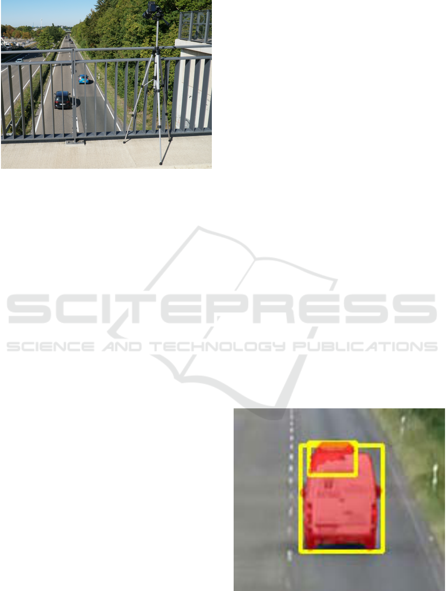
Figure 2: Photo of the recording setup. The camera is posi-

tioned on a tripod on a bridge and records the passing trafﬁc

from behind.

for this non-instructed trafﬁc no ground truth is avail-

able, the positioning accuracy of the detections can

not be evaluated. Therefore, an additional reference

vehicle performs various maneuvers in the ﬁeld-of-

view of both recording systems. This reference ve-

hicle is equipped with a high-accuracy inertial navi-

gation system whose acquired trajectories serve for a

comparison.

The remaining chapters are structured as fol-

lows: Chapter 4 describes the implementation of the

infrastructure-based system. In chapter 5 an analyt-

ical identiﬁcation and comparison of the limitations

of relevant parameters for the quality of the resulting

datasets follows. The experiments in chapter 6 exam-

ine on the one hand the detection rates of both sys-

tems for non-instructed road users and on the other

hand the positioning accuracy of a reference vehicle

in both recordings.

4 CAMERA-BASED

INFRASTRUCTURE SENSOR

SYSTEM

The recording of trafﬁc participants and the con-

version to trajectories is a procedure that, like the

processing of drone-based trafﬁc recordings, is per-

formed in several disjunctive steps. Also, the process-

ing of the recordings is not performed live during the

recording.

For the recordings themselves a Sony Alpha 6300

with an 18 mm lens is used. The camera can record

videos in 4K resolution at 25 FPS and is positioned

on a tripod on a bridge as shown in Fig. 2. Thus, the

camera is located at a height of about 8.5 m above the

road. The camera ﬁlms the trafﬁc in portrait format

and is slightly angled so that the captured two-lane

road section covers as large an area of the camera im-

age as possible. The shots are limited to one of the

two driving directions because the middle shoulder is

full of trees blocking the view of the other lane. An in-

trinsic calibration of the camera minimizes distortions

caused by the imperfections of the recording device.

The ﬁrst processing step is the detection of all

trafﬁc participants in each frame of the recordings.

The state of the art has shown that neural networks

are suitable for this purpose. Since road users often

partially or completely overlap each other from the

chosen perspective, e.g. a simple semantic segmen-

tation is not sufﬁcient. Instead, instance segmenta-

tion is necessary, so that we use a Mask-RCNN (He

et al., 2017) network in accordance with the literature.

Although a Mask-RCNN pre-trained on COCO (Lin

et al., 2014) was already able to detect some vehicles

correctly, we have ﬁne-tuned the network using our

own training dataset. While public datasets as DE-

TRAC (Wen et al., 2020) were available, we needed a

dataset including instance segmentations for achiev-

ing the highest quality. The resulting network is able

to detect even partially covered vehicles at greater dis-

tances, as shown in Fig. 3.

The detection of the vehicles in the camera image

does not yet allow to determine their trajectories on

the 2D road surface. Beforehand, the position of the

vehicle on the road must be deduced from the position

of the detection in the image by a perspective map-

ping. While from the drone perspective only the per-

spective distortion caused by the three-dimensional

vehicle shape has to be considered, the camera per-

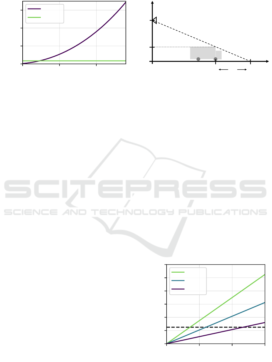
Figure 3: Examplary zoomed-in result of the Mask-RCNN

network ﬁne-tuned on our use-case. The results show that

even partially occluded vehicles are typically detected.

VEHITS 2021 - 7th International Conference on Vehicle Technology and Intelligent Transport Systems

164

0 m 10 m 20 m 30 m 40 m 50 m

60 m

0 m

10 m

20 m

30 m

60 m

Figure 4: Visualization of the image mapping. While in the left image an original, untransformed frame is shown, the right

image shows the mapped result. The red line indicating the distances to the camera shows that the perspective is removed

from the mapped image. However, with increasing distance, the resolution decreases.

spective from the infrastructure sensors has to be con-

sidered here as well. Since the vehicle height has little

relevance for a trajectory dataset and the considered

road section can be assumed to be almost horizontal,

an omission of the third dimension is possible. To de-

termine the mapping, salient points in the camera im-

age and in an orthophoto are matched. The mapping

not only corrects the perspective but also converts pix-

els into meters. In Fig. 4, this is done exemplary for

a camera image, although only the detections them-

selves have to be mapped. The length and width of

each vehicle are measured when entering the image

since this is where the least perspective distortion is

present (compare Fig. 5). To determine the width of

the detected vehicles at this point, only the lower part

of the vehicles’ detections close to the road is trans-

Figure 5: Visualization of the size estimation for the

infrastructure-based system. A vehicle entering the

recorded area is shown. The estimated size is visualized

as yellow bounding box.

formed in order to avoid perspective errors. However,

for length measurement, the entire detection is trans-

formed for cars. As the perspective distortion at be-

ginning of the recorded road section is still not negli-

gible for trucks, a length modiﬁcation factor of 0.71

is applied when transforming the trucks’ detections.

This factor is derived from multiple manual measure-

ments.

In a last step, the mapped detections in the indi-

vidual frames must be linked to trajectories. This

is done by the Hungarian algorithm (Kuhn, 1955),

which is used for the optimal assignment of detec-

tions to tracks based on their distances in each frame.

To smooth the positions in the last step and also to

derive the velocities and accelerations from the posi-

tions an RTS smoother (Rauch et al., 1965) is used.

5 THEORETICAL COMPARISON

Before conducting the experiments, we want to derive

theoretically which parameters and variables for the

two approaches considered represent the typical bot-

tlenecks with respect to the resulting dataset quality.

For this purpose, we consider the individual process-

ing steps and derive the expected accuracies or errors

for each detection and resulting trajectory at the end.

Since especially errors at the beginning of the pro-

cessing chain are carried through all subsequent pro-

cessing steps, we focus on them here. As the tracking

module at the end can be designed from very simple

to very complex, and must ultimately correct previ-

ous errors, we will consider this module only superﬁ-

cially.

Comparison of Camera-Equipped Drones and Infrastructure Sensors for Creating Trajectory Datasets of Road Users

165

0 50 100

x [m]

0.0

0.2

0.4

0.6

GSD [m]

ITS-S

Drone

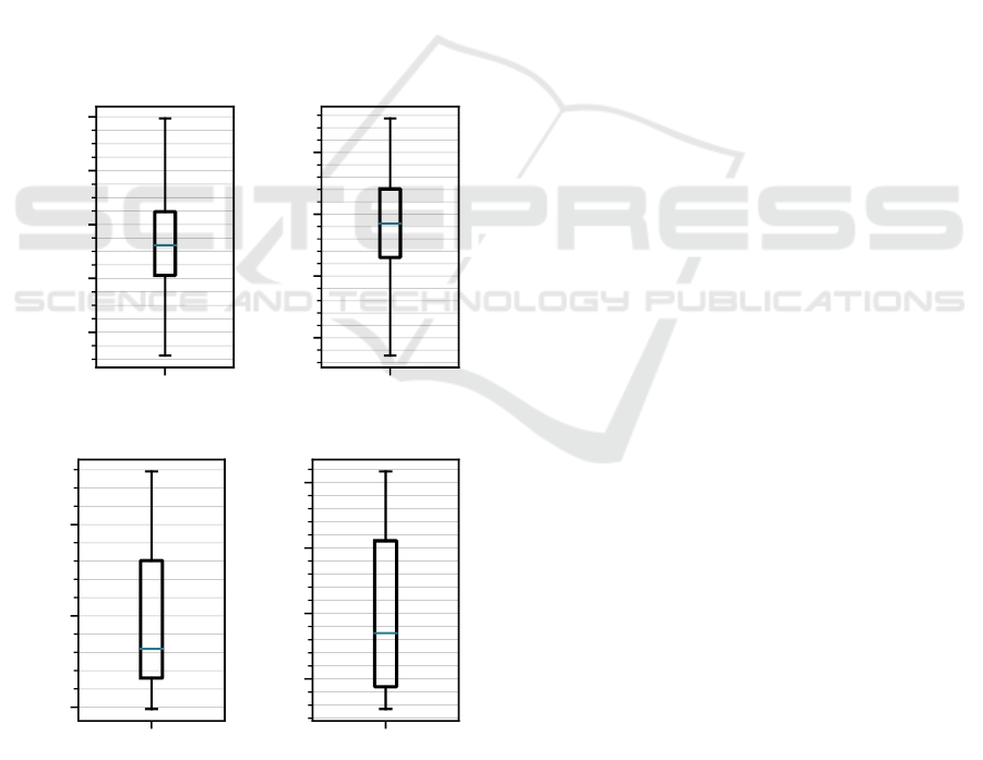
Figure 6: Comparison of the ground sampling dis-

tances (GSDs) between the drone-based (green) and the

infrastructure-based (violet) system.

Starting with the camera image itself, an elementary

difference becomes clear. The bird’s-eye view cap-

tures the entire road section under consideration with

a constant resolution or ground sampling distance

(GSD). At an altitude of 100 m a road section of up

to 140 m length is recorded with a ground sampling

distance of 3.4 cm/px at C4K resolution. In compar-

ison, the GSD for the stationary camera behaves ap-

proximately square from 0.005 m/px to 0.7 m/px at

the end of the image. As shown in Fig. 6, from 22 m

distance, the GSD is higher than for the drone. From

100 m distance, it is already 0.35 m/px.

The quality of the images themselves may also be

reduced by lens distortion and blurring. However,

we consider these errors to be negligible if the cam-

era has been calibrated correctly, and the exposure

time and aperture have been selected so that static and

dynamic content is sharply projected. With a shutter

speed of 1/500 s, from a bird’s eye view, the motion

blur of a vehicle with 70 km/h is only 0.04 m, which

is within the tolerance range of the GSD. From the

viewpoint of the stationary camera, the motion blur in

the close range is higher at the same exposure time,

but from about 20 m on it is signiﬁcantly smaller than

the GSD.

The ﬁnal recording-speciﬁc point are camera

movements. While the stationary camera is capturing

a ﬁxed street segment during a recording, the drone is

constantly moving slightly. These unavoidable move-

ments are caused, for example, by wind and too im-

precise sensors used to stabilize the hovering position.

This leads to a shift of the captured road section by up

to a few meters during a recording, which can be cor-

rected by the drone pilot. Further, the state of the art

has shown that resulting position errors of extracted

road users can be virtually eliminated by video stabi-

lization (Krajewski et al., 2018).

A theoretical comparison of the quality of the ob-

ject detection is difﬁcult. For both perspectives, a

Δx

Figure 7: Extent of vehicle-vehicle occlusions ∆x in a

camera-based ITS-S as a function of camera height h

, ve-

hicle distance x

, and vehicle height h

large repertoire of algorithms can be used. There-

fore the accuracy depends more on the amount of

annotations and the available computing time. A

non-quantiﬁable difference, however, is that from the

drone perspective the objects to be detected are of a

very similar size. On the other hand, in ITS-S-based

images, very large to very small, as well as partially

occluded objects must be detected.

Vehicle-vehicle Occlusions play an important

role in the detection process. Here, the drone has a

clear advantage, because if the drone is correctly posi-

tioned near or above the road, masking between vehi-

cles can be completely prevented. From the perspec-

tive of the stationary camera, however, occlusions

cannot be excluded. The extent of the occlusions de-

pends on the height of the camera, the vehicles and

the distances, as shown in Fig. 7. The occluded dis-

tance can be derived as ∆x = (h

· x

)/(h

− h

). As

depicted in Fig. 8, especially for vans and trucks (par-

tial) occlusions have to be expected assuming a fol-

lowing distance of 25 m at 70 km/h.

0 50 100 150

[m]

100

120

∆x [m]

Truck

Van

Car

Figure 8: Occluded distance ∆x over vehicle distance x

for

a camera mounted at h

= 8m. Results for car (violet, h

1.5m), van (blue, h

= 2.5 m) and truck (green, h

= 3.5 m).

VEHITS 2021 - 7th International Conference on Vehicle Technology and Intelligent Transport Systems

166

From the object detections both the object size

and the center to be tracked must be derived. Due

to the perspective, the stationary camera has clear ad-

vantages in estimating the vehicle height compared

to the drone. On the other hand, the vehicle length

can only be determined much less accurately as it en-

ters the image. Especially high trucks cover their own

driver’s cab (compare Fig. 4). From the drone per-

spective, the vehicle length and width can be deter-

mined most easily in the center of the image, since

the sides of the vehicle are hardly visible here. Ac-

cordingly, it makes sense to directly track the center

point as well as the orientation of road users from a

drone perspective, since no additional error is gener-

ated. From the bridge perspective, however, the ori-

entation cannot be estimated with the approach shown

and the object center can only be tracked indirectly

via the rear axle.

The GSD again plays a central role in the georef-

erencing of the detections. While drone images with

a GSD of 3.4 cm/px have a higher resolution than

orthophotos, the increasing GSD of stationary cam-

eras makes the georeferencing of pixels at greater dis-

tances more difﬁcult.

6 EXPERIMENTS

The two sensor systems are evaluated in two exper-

iments. At ﬁrst, we compare the general detection

statistics in order to obtain a general assessment of

the quality of both systems. This is done by analyz-

ing the tracks of all detected non-instructed road users

on properties that don’t require a ground truth since

no independent reference measurement is given for

those. In the second step, the localization accuracy of

both systems is tested against a reference vehicle with

an inertial navigation system.

In order to tempo-spatial synchronize all systems,

optical features were used for the drone and ITS-S.

While for the temporal synchronization the passing

of vehicle rears at unique keypoints was used, the

spatial synchronization was done by georeferencing

the recordings to an orthophoto in UTM coordinates.

Then, the recordings of the reference vehicle were

synchronized to the drone recordings by matching the

generated tracks and minimizing the error of all cen-

troids at all timesteps. A further spatial synchroniza-

tion was not necessary, since the INS of the reference

vehicle already outputs its position in UTM coordi-

nates. All synchronization steps were manually veri-

ﬁed.

0 100 200

Distance [m]

−2

Oﬀset [m]

Figure 9: Example ITS-S measurements of a vehicles’ x-

position offset to the ﬁltered position. The vehicle was driv-

ing at a nearly constant speed. The dashed lines indicate the

theoretical maximal accuracy a vehicle can be detected at

that distance (GSD).

6.1 Detection Statistics

In the chosen recording setup, the ITS-S’s ﬁeld of

view covered a road section of about 400 m. This sec-

tion length can also be covered by a drone, as shown

for the highD dataset (Krajewski et al., 2018). How-

ever, due to regulations, the ﬂight altitude was limited

to 100 m at the chosen recording site. As this reduced

the covered road section length to 140 m, we use only

this distance for comparison of both systems. For all

recordings, the drone was positioned to capture the

nearest 140 m to the ITS-S.

We recorded a total of 35 minutes on a sunny day.

During the recordings, 452 vehicles passed the mea-

surement sector. Both systems managed to initially

detect all of them. The tracks generated by the drone

recordings have an average length of 134.3 m. Con-

sidering that tracking only starts as soon as a vehi-

cle is completely visible in the image, the maximum

possible tracking distance is thus slightly smaller than

the recorded length of the road of about 140 m. This

means that (almost) all vehicles are tracked over the

entire distance. Similarly, the average track length

generated by the ITS-S recordings is 135.5 m, con-

sidering only the ﬁrst 140 m of the recorded road sec-

tion. Therefore, both approaches are able to reliably

track road users over 140 m. However, if the entire

road section visible to the ITS-S (400 m) is consid-

ered, the average track length is only 263.3 m. A

more detailed analysis of the tracks shows, that the

system often fails to detect vehicles at a greater dis-

tance from the camera. There are mainly two reasons

for this. Firstly, as seen in Fig. 6, the ground sampling

distance deteriorates quadratically with the distance.

Thereby the variance of the detections also increases

with the distance (see Fig. 9). If the variance turns

too great, the Hungarian algorithm may not be able

Comparison of Camera-Equipped Drones and Infrastructure Sensors for Creating Trajectory Datasets of Road Users

167

to correctly assign the detections to the correspond-

ing tracks. This leads ultimately to an end of the af-

fected track if this happens too often in consecutive

time steps. Secondly, about 21.5 % of the vehicles

are at least for one frame occluded by another vehi-

cle in the considered road segment. The chance for

this to happen rises with the distance to the camera as

seen in Fig. 7. Fully occluded vehicles can no longer

be detected and therefore no longer be tracked. In

contrast, a higher ﬂight altitude of the drone and thus

a larger area covered increases the ground sampling

distance, but not to a lower detection rate. The highD

dataset (Krajewski et al., 2018) shows that vehicles

are reliably detected even at signiﬁcantly higher ﬂight

altitudes.

Fig. 10 shows a comparison of the vehicle dimen-

sions, separated by the two detected classes. For cars,

the measured widths match to a great extent, with

a median deviation of only 1.5 cm. This indicates,

that both systems are able to accurately estimate this

value. Considering the length, the cars are typically

Length

−0.2

0.0

0.2

0.4

0.6

Deviation [m]

Width

−0.2

−0.1

0.0

0.1

(a) Car.

Length

0.0

0.5

1.0

Deviation [m]

Width

−0.1

0.0

0.1

0.2

(b) Truck.

Figure 10: Statistical evaluation of the measured dimension

differences between both systems. For each vehicle, the cal-

culated dimensions by the two approaches were subtracted.

A positive value indicates a higher value measured by the

ITS-S.

measured a bit too long by the ITS-S, with a median

deviation of about 12.5 cm. The main factor is pre-

sumably the diversely shaped car fronts, which can

distort the transformed detections of the ITS-S. For

systems, which measure the vehicles not only from

the back but also from different perspectives, this er-

ror could be eliminated.

The measured widths of trucks differ at a median

of about 0.03 cm. Since the ITS-S is recording vehi-

cles from behind, it is able to precisely determine the

trucks’ width. In case of the drone, perspective dis-

tortions of tall vehicles have to be considered. The

system we used is able to compensate for this effect

by assuming an average truck height of 3.50 m. Over-

all, the small deviations suggest that both systems can

reliably measure the width of trucks. Regarding the

length measurement, the ITS-S is only able to esti-

mate the length of the trucks (see section 4). This

leads to signiﬁcant deviations in the measurements of

the truck lengths. Due to the diverse truck shapes that

occur, it is not possible to completely eliminate this

effect.

6.2 Localization Accuracy

During the recordings, we passed the measurement

sector eight times with our reference vehicle. To in-

clude lateral movements, we performed a lane change

to simulate different scenarios in four of these passes.

Independently from that, we accelerated the vehicle in

three passes to incorporate the effect of varying speed

on the tracking into the evaluation. From the ITS-S

perspective, the vehicle became partially occluded in

two of those passes.

Fig. 11 shows an exemplary trajectory compari-

son of one pass. It is immediately noticeable that the

trajectory of the reference vehicle shows a deviation

from the other two trajectories. Our experiments have

shown that this is caused by a GPS drift perpendicu-

lar to the direction of motion, resulting from an erro-

neous GPS ﬁx after passing under a bridge. This drift

is not deterministic and couldn’t be compensated by

the differential GPS signal for our measurements, but

it averages to about 30 cm and is constant over the en-

tire course of a measurement. Apart from this, the

accuracy of the inertial navigation system is 1-2 cm

and thus maps the course of the trajectory with high

precision.

Analyzing the deviations of the drone and ITS-S

measurements over the distance results in the curves

shown in Fig. 12. As expected, the deviation of the

drone tracks is almost constant over the entire mea-

surement distance and varies in a range of only 2 cm,

which is consistent with the theoretically determined

VEHITS 2021 - 7th International Conference on Vehicle Technology and Intelligent Transport Systems

168

0 50 100

x [m]

y [m]

0 1 2 3 4

100

x [m]

0 1 2 3 4

t [s]

2.5

5.0

y [m]

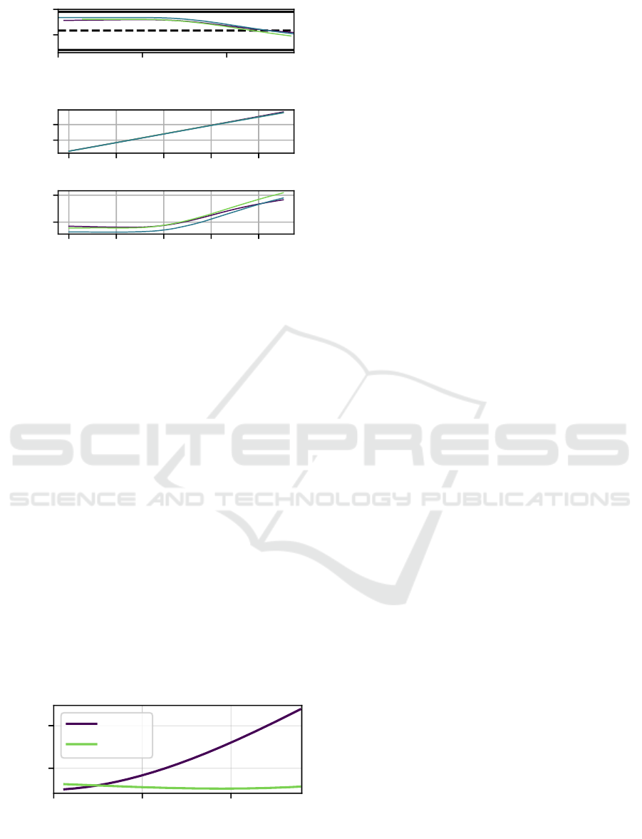
Figure 11: Exemplary trajectory comparison of the refer-

ence vehicle. The top graph shows the trajectories of the

ITS-S (violet), drone (green) and reference vehicle (blue)

from a bird’s-eye perspective. The two graphs below show

the positions in x- respectively y-direction over the time

where all three methods tracked the vehicle. The reference

vehicle became occluded from the ITS-S perspective after

around two seconds, which leads to a visible deviation in

the y-direction.

GSD. The minimum deviation for both measurement

methods is about 30 cm. This corresponds approxi-

mately to the value which we have determined as the

average GPS drift. Assuming an error-free reference

measurement, the minimum deviation would be re-

duced by the amount of the GPS drift, which results in

a convincing tracking performance by the drone over

the entire road section.

The ITS-S measurements also show the char-

acteristics as expected in chapter 5, but the abso-

lute degradation of the accuracy is signiﬁcantly lower

than that of the GSD. This can be explained by

the Kalman ﬁltering of the measurements during the

tracking, which results in an acceptable accuracy even

at greater distances. Compared to the drone, the ITS-

S achieves comparable or even better accuracy up to

0 50 100

x [m]

0.4

0.6

Deviation [m]

ITS-S

Drone

Figure 12: Averaged deviation from the reference measure-

ments. Due to the low sample size the curves are slightly

smoothed to compensate for the measurement variances.

a distance of 30 m. However, at longer distances, the

accuracy of the ITS-S can no longer keep up with the

drone due to the perspective.

7 CONCLUSION

In this paper, we have presented a comparison be-

tween two typical approaches to the creation of trajec-

tory datasets of road users. The analysis of the state

of the art has shown that trajectory datasets have an

increasing relevance for automated driving. The two

common approaches to create high-quality datasets

are the use of ITS-Ss and drones. However, there is

no concrete qualitative or quantitative comparison of

both methods in the literature so far. Therefore, we

have developed a camera-based infrastructure system

for the detection of road users from elevated positions

in accordance with the state of the art in order to com-

pare it with an existing drone approach. The theo-

retical analysis has shown that the biggest inﬂuence

on quality is the perspective as well as the ground

sampling distance. Within the experiments, we could

conﬁrm these results. Both systems were able to reli-

ably track vehicles over a course of 140 m. Consid-

ering greater distances though, the ITS-S struggled

due to vehicle-to-vehicle occlusions. Experiments

with a reference vehicle have shown that the position-

ing accuracy near the infrastructure system is at the

same level as the drone system, but decreases gradu-

ally from a distance of 30 m. In summary, we have

theoretically and experimentally shown that both ap-

proaches are able to detect all road users, although

drone-based systems have an advantage regarding the

distance independent road user localization accuracy.

ACKNOWLEDGEMENTS

The research leading to these results is further funded

by the Federal Ministry of Transport and Digital In-

frastructure (BMVI) within the project ”ACCorD:

Corridor for New Mobility Aachen - D

usseldorf”

(FKZ 01MM19001). The authors would like to thank

the consortium for the successful cooperation.

REFERENCES

Bock, J., Krajewski, R., Moers, T., Runde, S., Vater, L.,

and Eckstein, L. (2020). The ind dataset: A drone

dataset of naturalistic road user trajectories at german

intersections. In IEEE Intelligent Vehicles Symposium

(IVS).

Comparison of Camera-Equipped Drones and Infrastructure Sensors for Creating Trajectory Datasets of Road Users

169

Colyar, J. and Halkias, J. (2007). Us highway 101 dataset.

Federal Highway Administration (FHWA), Tech. Rep.

FHWA-HRT-07-030.

Cordts, M., Omran, M., Ramos, S., Rehfeld, T., Enzweiler,

M., Benenson, R., Franke, U., Roth, S., and Schiele,

B. (2016). The cityscapes dataset for semantic urban

scene understanding. In Proc. of the IEEE Conference

on Computer Vision and Pattern Recognition (CVPR).

Geiger, A., Lenz, P., Stiller, C., and Urtasun, R. (2013).

Vision meets robotics: The kitti dataset. International

Journal of Robotics Research (IJRR), 32(11).

He, K., Gkioxari, G., Doll

ar, P., and Girshick, R. (2017).

Mask r-cnn. Proceedings of the IEEE international

conference on computer vision, pages 2961–2969.

Houston, J., Zuidhof, G., Bergamini, L., Ye, Y., Jain, A.,

Omari, S., Iglovikov, V., and Ondruska, P. (2020). One

thousand and one hours: Self-driving motion predic-

tion dataset.

Kloeker, L., Kloeker, A., Thomsen, F., Erraji, A., and Eck-

stein, L. (2020). Trafﬁc detection using modular in-

frastructure sensors as a data basis for highly auto-

mated and connected driving. 29. Aachen Colloquium

- Sustainable Mobility, 29(2):1835–1844.

oster, F., Mazzega, J., and Knake-Langhorst, S. (2018).

Automatisierte und vernetzte systeme efﬁzient erprobt

und evaluiert. ATZextra, 23:26–29.

Krajewski, R., Bock, J., Kloeker, L., and Eckstein, L.

(2018). The highd dataset: A drone dataset of natural-

istic vehicle trajectories on german highways for val-

idation of highly automated driving systems. In 2018

21st International Conference on Intelligent Trans-

portation Systems (ITSC), pages 2118–2125.

Krajewski, R., Moers, T., Bock, J., Vater, L., and Lutz,

E. (2020). The round dataset: A drone dataset of

road user trajectories at roundabouts in germany. In

IEEE Intelligent Transportation Systems Conference

(ITSC).

ammer, A., Sch

oller, C., Gulati, D., Lakshminarasimhan,

V., Kurz, F., Rosenbaum, D., Lenz, C., and Knoll, A.

(2019). Providentia - a large-scale sensor system for

the assistance of autonomous vehicles and its evalua-

tion.

Kruber, F., Morales, E. S., Chakraborty, S., and Botsch, M.

(2020). Vehicle position estimation with aerial im-

agery from unmanned aerial vehicles. IEEE Intelli-

gent Vehicles Symposium IVS 2020.

Kuhn, H. W. (1955). The hungarian method for the assign-

ment problem. Naval Research Logistics Quarterly,

2:83–97.

Kurz, F., Waigand, D., Fouopi, P. P., Vig, E., Henry, C.,

Merkle, N., Rosenbaum, D., Gstaiger, V., Azimi,

S., Auer, S., Reinartz, P., and Knake-Langhorst, S.

(2018). Dlrad - a ﬁrst look on the new vision and map-

ping benchmark dataset. In ISPRS TC 1 Symposium,

pages 1–6.

Lin, T.-Y., Maire, M., Belongie, S., Hays, J., Perona, P., Ra-

manan, D., Doll

ar, P., and Zitnick, C. L. (2014). Mi-

crosoft coco: Common objects in context. In Fleet,

D., Pajdla, T., Schiele, B., and Tuytelaars, T., edi-

tors, Computer Vision – ECCV 2014, pages 740–755,

Cham. Springer International Publishing.

Rauch, H. E., Tung, F., and Striebel, C. T. (1965). Maxi-

mum likelihood estimates of linear dynamic systems.

AIAA journal, 3(8):1445–1450.

Robicquet, A., Sadeghian, A., Alahi, A., and Savarese, S.

(2016). Learning social etiquette: Human trajectory

understanding in crowded scenes. In European con-

ference on computer vision, pages 549–565.

Schnieder, L., Grippenkoven, J., Lemmer, K., Wang, W.,

and Lackhove, C. (2013). Aufbau eines forschungs-

bahn

ubergangs im rahmen der anwendungsplattform

intelligente mobilit

at. Signal und Draht (105), 6:25–

28.

Strigel, E., Meissner, D., Seeliger, F., Wilking, B., and Di-

etmayer, K. (2014). The ko-per intersection laser-

scanner and video dataset. In 17th International

IEEE Conference on Intelligent Transportation Sys-

tems (ITSC), pages 1900–1901.

Wen, L., Du, D., Cai, Z., Lei, Z., Chang, M.-C., Qi, H.,

Lim, J., Yang, M.-H., and Lyu, S. (2020). Ua-detrac:

A new benchmark and protocol for multi-object de-

tection and tracking. Computer Vision and Image Un-

derstanding.

Winner, H., Hakuli, S., Lotz, F., and Singer, C. (2015).

Handbuch Fahrerassistenzsysteme. Springer Vieweg,

Wiesbaden.

Yang, D., Li, L., Redmill, K., and Ozguner, U. (09.06.2019

- 12.06.2019). Top-view trajectories: A pedestrian

dataset of vehicle-crowd interaction from controlled

experiments and crowded campus. In 2019 IEEE

Intelligent Vehicles Symposium (IV), pages 899–904.

IEEE.

Zhan, W., Sun, L., Di Wang, Shi, H., Clausse, A., Nau-

mann, M., Kummerle, J., Konigshof, H., Stiller, C.,

de La Fortelle, A., et al. (2019). Interaction dataset:

An international, adversarial and cooperative motion

dataset in interactive driving scenarios with semantic

maps. arXiv preprint arXiv:1910.03088.

Zyner, A., Worrall, S., and Nebot, E. M. (2019). Acfr ﬁve

roundabouts dataset: Naturalistic driving at unsignal-

ized intersections. IEEE Intelligent Transportation

Systems Magazine, 11(4):8–18.

VEHITS 2021 - 7th International Conference on Vehicle Technology and Intelligent Transport Systems

170