Colorimetric Space Study: Application for Line Detection on Airport

Areas

Claire Meymandi-Nejad

1,2 a

, Esteban Perrotin

1,3

, Ariane Herbulot

1,4 b

and Michel Devy

CNRS, LAAS, Toulouse, France

INSA de Toulouse, Toulouse, France

AIRBUS OPERATIONS S.A.S., Toulouse, France

Univ. de Toulouse, UPS, LAAS, F-31400 Toulouse, France

Keywords:

Color Similarity, Features Extraction, Line Detection, Embedded Vision on Aircraft.

Abstract:

We propose an adaptive color reference reﬁnement process for color detection in an aeronautical application:

the detection of taxiway markings based on images acquired from an aircraft. Road markings detection is a key

functionality for autonomous driving, and is actively studied in the literature. However, few studies have been

conducted on aeronautics. Road markings are often detected by using color priors, sensitive to perturbations.

Color-based algorithms are still favored in this context as the markings color provides important information.

Our proposed method aims at reducing the impact of weather conditions, shadowing and illumination varia-

tions on color-based markings detection algorithms. Our approach adapts a given color reference in order to

deﬁne a new ﬂexible yet robust color reference while maximizing its difference to other colors in the image.

It is achieved through a statistical analysis of color similarity over a set of images, computed on several color

spaces and distance functions, in order to select the most relevant ones. We validate our approach by analyzing

the quantitative improvement induced by this method using two color-based markings detection algorithms,

based on the Hough Transform and the Particle Filter.

1 INTRODUCTION

Line detection provides one of the main information

required for ADAS (Advanced driver-assistance sys-

tems) or for autonomous driving. As such, it is widely

present in the automotive ﬁeld literature (Narote et al.,

2018). A good number of studies use a color and/or

contrast prior for line detection, where the color space

used for this application varies, such as L*a*b* (or

CIELAB) in (Kazemi and Baleghi, 2017), HSI in

(Sun et al., 2006) or HSV in (Lipski et al., 2008)

and (Mammeri et al., 2016). In the automotive ﬁeld,

markings are most of the time white, but their color

could vary following the type of road or country.

However, most of lane detection applications prefer

to convert color images to gray-scale images.

In the context of this study, we focus on aeronau-

tics. We are working on images provided by cam-

eras mounted both in the cockpit and on the tail ﬁn

of an aircraft; these images are obtained either from

https://orcid.org/0000-0002-2664-7684

https://orcid.org/0000-0002-8377-6474

a simulator or from a real aircraft while taxiing. We

aim to detect and track markings from each image in

order to feed scene understanding methods, such as

position and ego-motion estimation, required for au-

tonomous driving. In both domains, there are lines

of different colors with different meanings. Convert-

ing the image to a gray-scale representation could be

misleading and cause confusion, for instance between

white and yellow lines. This study concerns the air-

craft navigation on taxiways; in this case the color

of the markings to be detected is ’yellow’. In aero-

nautics, the reference color for the ’yellow’ markings

is deﬁned by the ICAO (International Civil Aviation

Organization) requirements (ICAO, 2018) in the xyz

color space by color ranges, only valid for a certain il-

lumination level. The yellow color is more difﬁcult to

detect than the white and can be easily confused with

green, red or light brown that can be found in the air-

port areas. We need to be able to describe accurately

the color differences and similarities of the pixels in

our image in order to best detect the markings.

Several studies have been conducted on color sim-

ilarity and invariance, with multiple color spaces deﬁ-

546

Meymandi-Nejad, C., Perrotin, E., Herbulot, A. and Devy, M.

Colorimetric Space Study: Application for Line Detection on Airport Areas.

DOI: 10.5220/0010456605460553

In Proceedings of the 7th International Conference on Vehicle Technology and Intelligent Transport Systems (VEHITS 2021), pages 546-553

ISBN: 978-989-758-513-5

nitions as listed in (Cheng et al., 2001), (Koschan and

Abidi, 2008) or (Madenda, 2005) where the author

presents color similarities between different shades

of yellow, based on several distance methods.For line

detection in automotive applications, the most widely

used color spaces are HSV, HSI and CIELAB, but in

this context, we encounter difﬁculties with the illumi-

nation and saturation of the markings color. With the

increase of computing resources and image databases,

these issues are increasingly addressed in the litera-

ture with the development of efﬁcient neural networks

such as (Karargyris, 2015) or (Chen et al., 2018) and

(Neven et al., 2018), where the ﬁrst one intends to

learn a transform towards a color space that will in-

crease the accuracy of the detection and the two others

are focusing on road markings detection. The article

(Gowda and Yuan, 2019) concludes that several color

spaces, such as RGB, CIELAB or HSV, might in-

crease the classiﬁcation result on speciﬁc classes and

that combining some of them could lead to a higher

accuracy. One of the objectives of this study is to de-

ﬁned which color space most represents the markings.

However, a previous study of the method proposed in

(Karargyris, 2015) has not offered satisfactory results

on some of our detection works. Also, solid model-

based non-linear transforms have been designed in

the literature to create complex color spaces mod-

els and we do not think that a CNN-based approach

will produce an outstanding transform for our prob-

lem. A major limitation to the use of neural networks

in our application is the lack of a consequent labeled

database. Several databases are available in the auto-

motive ﬁeld but qualitative databases do not exist in

aeronautics. This is why we are not currently basing

our research on solutions that use CNNs.

An additional difﬁculty when working with color

detection for automotive ﬁelds or aeronautical ap-

plications comes from the outdoor conditions. The

markings colors on the images are affected by shad-

owing, lightness variation, glare and other impacts of

the weather conditions, so that it is mandatory to in-

tegrate, in a line detection algorithm, a ﬂexible def-

inition of the reference color for markings. Those

perturbations change greatly the color of the mark-

ings that diverges from the ICAO requirements and

impacts negatively the markings detection.

In this article, in order to improve the detec-

tion of the yellow markings in any weather condi-

tion, we propose a data-driven method to adapt a

given color reference to segregate it in a given con-

text, based on a statistical analysis of the similar-

ity of colors with respect to the reference (here, the

ICAO color deﬁnition), using several color spaces

and color distance functions that we call pairs

(ColorSpace,DistanceMethod). We validate this

method using two color-based markings detection al-

gorithms, by measuring the quantitative improvement

of using the chosen pair. We show that our method

increases the robustness of the color segregation to

variations in illumination, resulting in a better seg-

mentation on the markings and the tarmac or grass

areas, thus a better detection. We chose to focus on

the yellow color markings, but this study can be gen-

eralized by changing the color reference (for instance

the red, white or blue marking colors deﬁned by the

ICAO requirements) and recalculating the color dis-

tances for each pair. This method can also be used in

applications beyond aeronautics context.

In Section 2, we propose a method to reﬁne a

color reference by minimizing the distance between

this reference and the actual pixels in an image. In

Section 3, we analyze several color distance functions

in several color spaces, in order to select the most rel-

evant pairs to discriminate a chosen color (here, the

ICAO yellow) from others. Section 4 proposes to use

the results of this analysis to tune the parameters of

the adaptive reﬁnement algorithm. This algorithm is

evaluated in Section 5. Finally, we compare two line

detection algorithms with and without the automatic

reference reﬁnement in Section 6 before concluding

about the applicability of the proposed method.

2 COLOR DISTANCE

COMPUTATION USING

ADAPTIVE REFERENCE

This section presents an algorithm to adapt a color

reference to a set of images in order to improve the

color segmentation. Since a lot of model-based line

detection algorithms are using either binary maps or

distance maps, which computation is mostly based on

a color processing, the choice of the color reference

has a great impact on the ﬁnal result.

We start from the ICAO color deﬁnition that de-

ﬁnes the color of the airport markings as a subset of

the xyz color space. It is then possible to select a

threshold to extract most of the lines from the image.

However, images used for this comparison are deﬁned

in the sRGB space, while the reference is deﬁned on

the full xyz space with speciﬁc illumination. Due to

evironment perturbations or sensors post-treatments,

the color of the markings is sure to vary from this ref-

erence color. Hence, we need to apply an empirical

modiﬁcation of this deﬁnition, to make it ﬂexible yet

as close as possible to the ICAO requirements.

We note C

∗

= {0.45,0.45,0.08}

xyz

the ideal color

Colorimetric Space Study: Application for Line Detection on Airport Areas

547

of the line. We denote

C the estimator of C

∗

on the ac-

tual image.

C is computed using a p-Nearest Neigh-

bors algorithm, presented in Algorithm 1. This algo-

rithm requires three parameters: C

∗

, p the size of the

considered neighborhood, and tolerance which de-

ﬁne the end criterion. A fourth parameter, thresh, is

needed to compute the binary map.

Algorithm 1: Color distance computation using adaptive

reference.

Require: p, image, C

∗

, tolerance, thresh

i = 0

di f f = in f

= Convert2ColorSpace(C

∗

)

image = Convert2ColorSpace(image)

while di f f > tolerance do

i = i + 1

dist = Distance(image,

i−1

))

~x = GetImageIndexes(sort(dist))

∑

k=1

(image(~x

))

di f f = Distance(

i−1

)

end while

dist = Distance(image,

))

bin = BinarizeDistanceMap(dist,thresh)

return

, dist, bin

Before using this algorithm, a Gaussian blur can

be performed on the image to remove possible outliers

with emphasis on a spatial constraint on the different

pixels. It is also used for noise reduction. The pro-

posed algorithm is composed of several steps. Firstly,

the RGB color space is not the most efﬁcient color

space for color comparison and is not overly used in

the literature where HSV and CIELAB color spaces

are favored. That is why we perform a conversion to

another color space before using the distance func-

tion, for example an Euclidean distance. As a result,

we obtain a gray-scale image representing the dis-

tance map dist. In order to reﬁne the reference color,

we need to select the pixels that provide the smallest

distance value to the reference color. For this pur-

pose, we create a vector of the distances contained in

the distance map and select a small number of those

pixels deﬁned by p. The new reference color is then

updated by the average color of the selected pixels.

Those functions are repeated until the color difference

between two colors is lesser than the tolerance. Fi-

nally after this algorithm, the binary map is obtained

by thresholding the distance map.

As we work on images that can suffer from the

weather conditions or shadowing, we need to ﬁnd a

ﬂexible algorithm that performs well on any image.

Hence selecting parameters suitable for any situation.

In the following section, we ﬁrst work on the pairs

(ColorSpace,DistanceMethod) to ﬁnd those that will

maximize the discrimination between the reference

color and the yellow hues on one part and any other

color in the image on the other part in order to se-

lect the best distance function to compute the distance

map. The selection of the parameters is presented in

Section 4 and is dependent on the Section 3 results.

3 STUDY OF COLOR SPACES

AND DISTANCE METHODS

This section proposes a statistical analysis of several

color representations to select the most relevant ones.

The color spaces and associated distance functions

considered are described in Table 1.

3.1 Notations

For the rest of this article, for the sake of readability,

we will use a common nomenclature for all color dis-

tance functions. In addition to the ones referenced in

Table 1, we note ’∆E

’ the Euclidean distances

between elements of a given color space, and ’∆E

’

or ’∆E

’ the Euclidean distance computed on a sub-

set of the channels. For instance, we write ∆E

the

Euclidean distance on the A and B channels of the

CIELAB color space, or ∆E

for the Hue channel

of the HSV color space. We also note ’∆C

LCH

’ the

weighted Euclidean distance for the LCH color space

given by Equation 1, where ∆L and ∆C are the dif-

ference between, respectively for the L and C chan-

nels, the reference and pixel colors (subscripted

re f

and

pix

), and δH is a combination of the information

given by the C and H channels of the colors.

∆C

LCH

(∆L)

+ (∆C)

+ (δH)

(1)

where δH =

re f

∗C

pix

∗ 2 ∗ sin(

pix

− H

re f

) (2)

Table 1: List of color spaces and distances selected for this

study, with commonly used notations in parenthesis.

Color Space Distances

HSV, HSL, XYZ,

YCbCr, YIQ

Euclidean distance on all channels

Euclidean distance on combinations of channels

RGB

Euclidean distance on all channels

Weighted Euclidean distance on all channels (∆C)

CIELAB

Euclidean distance on all channels (∆E∗

)

Euclidean distance on combinations of channels

CIE 1994 (∆E∗

)

CIE 2000 (∆E∗

)

L*C*h

Euclidean distance on all channels

Euclidean distance on combinations of channels

CMC l:c 1984 (∆E∗

CMC

)

Weighted Euclidean distance on all channels

VEHITS 2021 - 7th International Conference on Vehicle Technology and Intelligent Transport Systems

548

To select the distance function that best segregate

the color of the markings, we need to study the re-

sults of several pairs (ColorSpace, DistanceMethod).

We call ’color difference’ the result of the nor-

malized distance between a color and the refer-

ence color provided by the ICAO requirements

for a speciﬁc pair (ColorSpace, DistanceMethod) as

color di f f erence = ||d

i,E

(Re f , PixelColor)||, where

i is the distance method and E

the color space. Some

distance methods being deﬁned only for speciﬁc color

spaces. The distances are normalized by dividing the

color differences by the greatest color difference to

the ICAO reference color obtained for each pair.

3.2 Database Construction

In order to perform this study on the different dis-

tance functions, we decided to create a color database

using few real and simulated images provided by an

airport simulator. We work with eight images of

size 1280pX960p, four images come from cameras

mounted on an aircraft and four images come from a

simulator. Half of the real and simulated images come

from a camera mounted near the cockpit of the air-

craft ant the other half come from a camera placed in

the ﬁn of the aircraft. Among the eight images, three

present degraded weather conditions (fog, dusk, low

illumination). All the images are chosen at different

areas in the taxiway, with different marking patterns,

more or less complex.

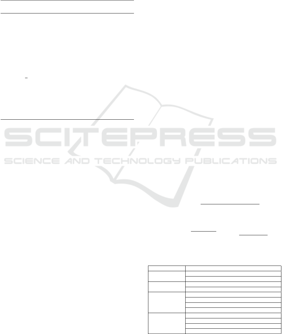
We ﬁrst analyzed the numerous colors present on

the selected images. The images can be separated in

areas, such as the taxiway (containing most of the

gray pixels), the sky (where the majority of the pix-

els are blue or light colors) and the grass around the

taxiway. Most of the colors encountered in the im-

ages can be simpliﬁed as either ’blue’, ’gray’, ’green’,

’red’, ’black’ (or dark colors), ’white’ (or light colors)

or ’yellow’ for the markings. We created a database

with the unique {R,G,B} triplet of pixels from simu-

lated and real images on several weather conditions,

in order to separate the image pixels in different color

classes and analyze the performance of all the pairs

(ColorSpace,DistanceMethod) in the segregation of

the markings color.

As the grass area is composed of a large amount

of different colors (green, yellow and brown for ex-

ample), we deﬁned two subclasses of colors in our

classiﬁcation that we call ’green’ and ’grass’. Fig-

ure 1 shows an example of one of the images and

corresponding masks for the labeling of the pixels

for the database. Figure 2 presents the classes that

we used for this study and their average proportion

in the database and in the images used to construct

the database. The colors are ordered by their values

on R then G and B. The ’undeﬁned’ class represents

RGB pixels that have been deﬁned as part of at least

2 classes depending on the images.

3.3 Statistical Analysis

We then decided to use multiple criteria to select a

subset of candidate pairs that best discriminate the

yellow class from the other classes, improving the

markings detection:

• The precision for a recall of 100%.

• The precision, recall and F

score.

• The dispersion and skewness of the color differ-

ences in each class.

Table 2 presents the results of the different pairs

based on those criteria for only 18 pairs out of 37.

The represented pairs have obtained at least a + on

one of the criteria with the exception of ∆E

that we

selected for its results on the box plot (see Figure 3)

and also because it is often used for the detection of

lines in the literature. From Table 2, we can select

three types of methods: those which mostly obtained

+ on the criteria (such as ∆E

or ∆E∗

CMC

), those

which obtained a mix of + and = (such as ∆E

∆E∗

) and those which obtained few + and mostly

= or − (such as ∆E∗

or ∆E

HSL

For the line Dispersion and Skewness, the + value

represents pairs which ensure that at least 75% of the

color differences of the yellow class can not be con-

fused with another class, the = value represents pairs

that could produce a confusion between the yellow

class and the gray, red, green or grass classes and the

− value lists the pairs which can not be used to segre-

gate the yellow class. In Figure 3, we present a sub-

set of the repartition of the color differences of the

cited colors for several pairs. The blue square corre-

sponds to the 25th and 75th percentile and the red line

is the median. The lower and upper adjacents (min-

imum and maximum values that are not considered

as outliers) values are given by the black whiskers

and the red crosses are the outliers, with their values

corresponding to more than 1.5 times the interquar-

tile range. The dotted and dashed lines represent the

thresholds reached for the upper adjacent and the 75th

percentile of the yellow class.

Figure 3 presents an example of box plot for three

pairs: ∆E

xyz

, ∆E

CbCr

and ∆E

that represent 3 sort of

results obtained for the 37 pairs. We can see that ∆E

xyz

can not be used to discriminate the yellow from the

other colors even though it is the color space where

the reference color for markings is deﬁned, empha-

sizing our need to ﬁnd a method to discriminate the

reference and yellow colors from other colors in the

Colorimetric Space Study: Application for Line Detection on Airport Areas

549

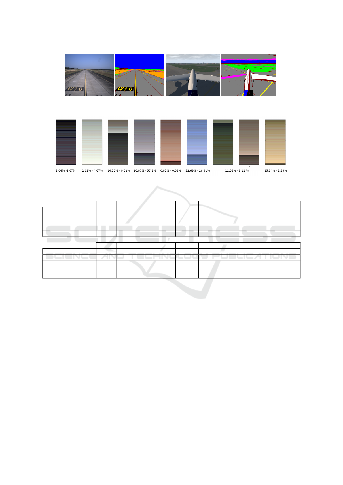
Figure 1: Example of building the database from real and simulated images. Each color mask correspond to one class, with

brown for unlabeled pixels, magenta for pixels labeled in several classes and orange for the grass class.

Figure 2: Classes Dark, Light, Undeﬁned, Gray, Red, Blue, Green, Grass and Yellow of the database. Below are the percent-

ages of the representation of the classes (database - image).

Table 2: Comparative table of the performances of several color spaces and distance functions.

∆E∗

∆E

∆E∗

∆E

LCH

∆C

LCH

∆E

∆E∗

CMC

Precision for Rec

100%

= + + + - - + - +

Precision for Rec

95%

= + + - - = = + +

Recall for Prec

95%

+ + + - + + + + +

Score + + + = + + + + +

Dispersion & Skewness + + + = + = = = +

∆E

HSV

∆E

HSL

∆E

(HSL/HSV) ∆E

YCbCr

∆E

CbCr

∆E

Y IQ

∆E

Precision for Rec

100%

- - - - + + - + -

Precision for Rec

95%

- - = - + + - = =

Recall for Prec

95%

= = - = + + = = -

Score + + = + + + + + +

Dispersion & Skewness - - = - = + - = -

image. Some pairs seem to allow the segregation of

the yellow color from others, such as ∆E

CbCr

as most

of the classes obtain color differences greater than the

75th percentile of the yellow class. We note that the

range of the color difference results is narrower for

those methods. However, the yellow class is closely

followed by the color differences results from the red

and grass classes. For the line detection, it could be a

problem as red markings have a completely different

meaning than yellow ones and we should avoid the

confusion. ∆E

(on the HSV or HSL color spaces)

has a small range of color difference results for the

yellow, red, grass and blue classes and can be used

to segregate the yellow color. However it also pro-

duces a great number of outliers for each class. Those

results are consistent with the large shade of hues of

each class as can be seen in Figure 2.

Based on the results from Table 2 and Figure 3,

we selected a subset of these pairs that we will vali-

date on images that have not been used to create the

database:

• ∆E∗

, ∆E

and ∆E∗

• ∆E

LCH

, ∆E

, ∆E∗

CMC

and ∆C

LCH

• ∆E

CbCr

, ∆E

(HSV/HSL)

4 TUNING OF THE ADAPTIVE

ALGORITHM PARAMETERS

Algorithm 1 needs three parameters: p, toler ance and

thresh. We propose to use the results of the color anal-

ysis in Section 3 to ﬁx these parameters.

Figure 2 shows that the colors of the markings rep-

resent an average of 1,39% of the pixels in an image,

we decided to ﬁx p as 0.1% of the average ratio of the

markings colors. This percentage enables us to select

enough pixels to compute a new reference color while

VEHITS 2021 - 7th International Conference on Vehicle Technology and Intelligent Transport Systems

550

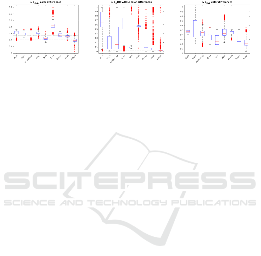
Figure 3: Box plot graphs representing the distribution of the color differences by class for several color spaces and distance

functions.

minimizing the probability of selecting outliers from

other classes that could degrade the reference color.

The purpose of the parameter thresh is to cre-

ate a binary map for the line detection algorithms.

To choose how to ﬁx its value, we used the study

of the precision, recall and F

score of the pairs

(ColorSpace,DistanceMethod). A ﬁrst idea was to

use the threshold for which we obtain the best F

score in the database analysis. While this threshold

maximizes the compromise between precision and re-

call, it can add outliers to the selection. In this speciﬁc

context, we decided to use the threshold which corre-

sponds to the loss of the maximum precision, prior-

itizing the precision over the recall, to minimize the

number of selected outliers. Unfortunately, this also

leads to a potential increase of the false negatives in

the pixels that represent a marking in the image.

The binary map obtained by the thresholding of

the distance map is used to analyze the possible num-

ber of pixels representing the markings in the image.

If the number of detected pixels in the binary map is

smaller than p, the algorithm will encounter difﬁcul-

ties to converge to a meaningful reference color. The

reﬁnement of the reference color is performed while

the color difference is lesser than tolerance.

5 EVALUATION OF THE

ADAPTIVE ALGORITHM

Thanks to the database study, we selected sev-

eral pairs as candidates for the distance function

in Algorithm 1. We decided to compute the dis-

tance and binary maps using each candidate pair

(ColorSpace,DistanceMethod) on images not used in

the database, both simulated and real, with different

weather conditions. The comparison is computed on

eight images, selected with the same ratio as the im-

ages used for the creation of the database. The binary

map is computed by using the parameter thresh se-

lected in Section 4.

Figure 4 presents binary and distance maps results

for different pairs on a ﬁn camera image and a com-

parison with the ground truth (last image of the sec-

ond row). The results of ∆E∗

CMC

, ∆E∗

, ∆E

LCH

∆E∗

and ∆E∗

(HSV/HSL) stand out compared to

others. Mostly, any distance method applied to the

L*C*h color space gives tangible binary maps.

Table 3 provides results on the precision, recall,

score and accuracy of the binary maps compared

to the ground truth, with a reﬂexion on computation

time. The results represent a mean value of the results

of the validation images. Several groups of methods

appear in Table 3. ∆E∗

CMC

and ∆E

LCH

show good

results on the different criteria. ∆E∗

, ∆C

LCH

, ∆E

and ∆E

obtain average results where the other meth-

ods are not satisfactory. However the computational

time can be an important factor in applications.

As expected, methods with small computational

time have worst results than methods with high or

average computational time. ∆E∗

CMC

is the better

choice if the computation time is not an important fac-

tor but for real time applications ∆E

LCH

is a good sub-

stitute. ∆E

could be selected for high speed compu-

tation. We could update the reference color only every

second to reduce the impact of the computation time

on the selection of the distance function.

When analyzing the color difference to the refer-

ence for each class deﬁned in this application, we es-

timated the precision of the pairs to discriminate the

’Yellow’ class. However, we have a representative-

ness bias in the database because the proportion of

each class in the database is different from their pro-

portion in the images, as the triplets’ colors are unique

in the database. It means that a color of a pixel deﬁned

as ’outlier’ in the ’gray’ class can be labeled as ’Yel-

low’ without a great impact on the pair results.

It could represent a big part of the taxiway in

the image and modify the performances between the

database study and the reference color selection re-

sults. This explains why several pairs provided good

results during the database study while their resultant

Colorimetric Space Study: Application for Line Detection on Airport Areas

551

Figure 4: Example of Binary (left) and Distance (right) maps for ﬁn camera images. First line: ∆E∗

, ∆E

, ∆E∗

Second line: ∆E

LCH

, ∆C

LCH

, ∆E

, ∆E∗

CMC

, ground truth. Third line: ∆E

CbCr

, ∆E

(HSV/HSL).

Table 3: Comparative table of several color spaces and distance functions on test images (not used in the database).

∆E∗

∆E

∆E∗

∆E

LCH

∆C

LCH

∆E

∆E∗

CMC

∆E

CbCr

∆E

Precision - - - = = - - + - - - +

Recall = + + - = = = = + + + -

score - - - + + = = + - - - -

Accuracy = - - + + = + + - - - +

Computation time = = = = = = = - + + + +

Table 4: Results of line detection algorithms with and without the adaptive reﬁnement of the reference color.

Recall Mean Dist Max Detection

HT PF HT PF HT PF GT

cockpit 0.9 0.92 0.14 5.22 394 397 607

cockpit adapt. ref. 0.94 0.96 3.07 0.71 536 565 607

ﬁn 0.34 0.61 11.73 59.02 326 357.7 810.56

ﬁn adapt. ref. 0.58 0.86 6.95 5.94 705 618.5 810.56

distance and binary maps are not satisfying. We could

add a weight to our dataset colors to increase the ro-

bustness of the classiﬁcation or add multiples entries

of the same (R,G,B) triplets in order to correct this

bias partially. We decided to keep this bias in the

database and take it into account in the second part

of the pairs selection when testing the pairs on global

images.

Following the results of Table 3, we decided to

select ∆E∗

CMC

. We can note that ∆E∗

gives good

results for the binary map. It also gives better results

for the distance map than ∆E∗

CMC

as the contrast be-

tween pixels corresponding to the markings and the

other pixels is greater. However, this method is less

robust on our images.

6 QUANTITATIVE VALIDATION

ON LINE DETECTION

ALGORITHMS

In order to validate this study, we decided to compare

the results for two line detection algorithms: a method

based on the Hough Transform as presented in (Hota

et al., 2009), called HT in Table 4, and a Particle Filter

(PF) implementation (Meymandi-Nejad et al., 2019),

on real images only. Both use a color assumption.

In order to compare the results of the line detection

algorithms with and without using Algorithm 1, we

decided to base this analysis on three criteria:

• Maximum Range of Detection (in Pixels): One

of the difﬁculties with our images is that, for ﬁn

camera images, the important lines can be found

at at least 50 meters from the camera. At this

point, the color of the markings is prone to noise

and additional saturation which increases its dif-

ference from the reference color.

VEHITS 2021 - 7th International Conference on Vehicle Technology and Intelligent Transport Systems

552

• Mean of the Clusters’ Pixels’ Distances to the

Ground Truth: it is used as a measure of the al-

gorithm precision. It computes, for each group of

pixels, the distance between the potential pixels

representing a marking and the ground truth.

• Recall.

Table 4 shows that all the metrics are improved for

both methods by using the adaptive research of the

markings reference color. In particular, we note a

signiﬁcant increase in the maximum detection range.

The results are more important on the ﬁn camera im-

ages because the lines are more blurred and easily

confused with the tarmac, particularly when they are

far from the camera. We also note an increase of the

maximum range detection, directly linked to a better

separation between the tarmac and the line.

7 CONCLUSIONS

In this paper, we evaluated several distances be-

tween a reference color and pixels of an image, us-

ing multiple color spaces, in order to deﬁne the pair

(ColorSpace,DistanceMethod) that best separate the

markings color from the rest of the image. We pre-

sented an algorithm to automatically reﬁne this refer-

ence color, required for the detection of markings in

airport areas. We computed the distance between the

reference color and the color of every pixel in the im-

age, providing either a binary image with pixels clas-

siﬁed as ’markings’ or a distance map; these outputs

are exploited by two line detection algorithms, based

on the Hough transform or the Particle Filter. We ob-

served a clear improvement of their results when us-

ing the adaptive reﬁnement of the reference color.

Such a method can be used, for instance, to de-

tect several markings in the airport areas such as bea-

cons or other colors of lines by modifying the refer-

ence color and re-running the database and robust-

ness to noise studies. Assuming the use of neural

networks on a prospective study, it could be interest-

ing to compare the results of changing the RGB im-

age to a L*C*h image as an input of the network on

the detection results. In this study, we worked with

known color spaces without deﬁning an order relation

between their channels. Future works could include

an algorithm as proposed in (Lambert and Chanus-

sot, 2000), to improve the yellow boundaries detec-

tion process while adding an order relation between

the channels of the different color spaces. It could

also be interesting to use CNNs to deal with more

complex classiﬁcations such as non-linear separators,

taking into account the concerns about the certiﬁca-

tions problems.

REFERENCES

Chen, P., Lo, S., Hang, H., Chan, S., and Lin, J. (2018).

Efﬁcient road lane marking detection with deep learn-

ing. In 2018 IEEE 23rd International Conference on

Digital Signal Processing (DSP).

Cheng, H., Jiang, X., Sun, Y., and Wang, J. (2001). Color

image segmentation: Advances and prospects. Pattern

Recognition.

Gowda, S. N. and Yuan, C. (2019). Colornet: Investigating

the importance of color spaces for image classiﬁca-

tion. In Computer Vision – ACCV 2018.

Hota, R. N., Syed, S., Bandyopadhyay, S., and Krishna,

P. R. (2009). A simple and efﬁcient lane detection us-

ing clustering and weighted regression. In COMAD.

ICAO (2018). AERODROMES: aerodromes design and op-

erations.

Karargyris, A. (2015). Color space transformation network.

arXiv.

Kazemi, M. and Baleghi, Y. (2017). L*a*b* color model

based road lane detection in autonomous vehicles. In-

telligent Transportation Systems (ITS).

Koschan, A. and Abidi, M. (2008). Digital color image

processing. John Wiley & Sons.

Lambert, P. and Chanussot, J. (2000). Extending mathe-

matical morphology to color image processing. Proc.

CGIP.

Lipski, C., Scholz, B., Berger, K., Linz, C., Stich, T., and

Magnor, M. (2008). A fast and robust approach to lane

marking detection and lane tracking. IEEE Southwest

Symposium on Image Analysis and Interpretation.

Madenda, S. (2005). A new perceptually uniform color

space with associated color similarity measure for

content-based image and video retrieval. Multimedia

Information Retrieval Workshop, 28th Annual ACM

SIGIR Conference.

Mammeri, A., Boukerche, A., and Tang, Z. (2016). A real-

time lane marking localization, tracking and commu-

nication system. Computer Communications.

Meymandi-Nejad, C., Kaddaoui, S. E., Devy, M., and Her-

bulot, A. (2019). Lane detection and scene interpreta-

tion by particle ﬁlter in airport areas. In International

Conference on Computer Vision Theory and Applica-

tions.

Narote, S. P., Bhujbal, P. N., Narote, A. S., and Dhane,

D. M. (2018). A review of recent advances in lane de-

tection and departure warning system. Pattern Recog-

nition.

Neven, D., Brabandere, B. D., Georgoulis, S., Proesmans,

M., and Gool, L. V. (2018). Towards end-to-end lane

detection: an instance segmentation approach. IEEE

Intelligent Vehicles Symposium.

Sun, T.-Y., Tsai, S.-J., and Chan, V. (2006). Hsi color model

based lane-marking detection. IEEE Intelligent Trans-

portation Systems Conference.

Colorimetric Space Study: Application for Line Detection on Airport Areas

553