
Global Reward Design for Cooperative Agents to Achieve Flexible
Production Control under Real-time Constraints
Sebastian Pol
1
, Schirin Baer
2
, Danielle Turner
1
, Vladimir Samsonov
2
and Tobias Meisen
3
1
Siemens AG, Digital Industries, Nuremberg, Germany
2
Institute of Information Management in Mechanical Engineering, RWTH Aachen University, Aachen, Germany
3
Institute of Technologies and Management of the Digital Transformation, University of Wuppertal, Wuppertal, Germany
vladimir.samsonov@ima.rwth-aachen.de, meisen@uni-wuppertal.de
Keywords:
Cooperative Agents, Deep Reinforcement Learning, Flexible Manufacturing System, Global Optimization,
Job Shop Scheduling, Reactive Scheduling, Reward Design.
Abstract:
In flexible manufacturing, efficient production requires reactive control. We present a solution for solving
practical and flexible job shop scheduling problems, focusing on minimizing total makespan while dealing
with many product variants and unseen production scenarios. In our system, each product is controlled by an
independent reinforcement learning agent for resource allocation and transportation. A significant challenge
in multi-agent solutions is collaboration between agents for a common optimization objective. We implement
and compare two global reward designs enabling cooperation between the agents during production. Namely,
we use dense local rewards augmented with global reward factors, and a sparse global reward design. The
agents are trained on randomized product combinations. We validate the results using unseen scheduling
scenarios to evaluate generalization. Our goal is not to outperform existing domain-specific heuristics for total
makespan, but to generate comparably good schedules with the advantage of being able to instantaneously
react to unforeseen events. While the implemented reward designs show very promising results, the dense
reward design performs slightly better while the sparse reward design is much more intuitive to implement. We
benchmark our results against simulated annealing based on total makespan and computation time, showing
that we achieve comparable results with reactive behavior.
1 INTRODUCTION
In today’s flexible manufacturing, reactive production
control is a key component for efficient production. It
is necessary to deal with increasing levels of uncer-
tainty introduced by the dynamic nature of complex
manufacturing setups and self-planning technologies.
Therefore it becomes vital to respond to unforeseen
events such as machine failures and demand fluctu-
ations with low decision-making latency while en-
suring the minimum negative impact on the produc-
tion as a whole. Every adjustment in planning has to
consider common objectives accomplished by all en-
tities in the system, such as minimization of the to-
tal production makespan, low inventory levels, and
high schedule adherence. This allows us to define
three main requirements for scheduling systems de-
ployed in flexible manufacturing: (1) fulfilling global
scheduling optimization goals, (2) fast reaction to un-
foreseen events, and (3) dealing with a large number
of product variants. It should be mentioned that most
heuristics solving the Job Shop Scheduling Problem
(JSSP) cannot cope with the named requirements, as
they are neither reactive during production, nor to new
products without adaptation. Therefore we concen-
trate on enabling reactive scheduling for flexible man-
ufacturing while ensuring results which are compara-
ble to the performance of common heuristics with low
computation times. To fulfill those requirements we
propose a Reinforcement Learning (RL) system capa-
ble of solving practical and flexible JSSPs. Designing
a Multi-Agent RL (MARL) scheduling solution for
all three tasks goes far beyond the classical JSSP and
has barely been studied within the past years. For this,
we adapt the approach of (Baer et al., 2020b) where
production and transportation of each product is con-
trolled by a separate RL agent. This work concen-
trates on achieving an improved fulfillment of com-
mon optimization objectives as formulated in the first
requirement by improving cooperation between the
Pol, S., Baer, S., Turner, D., Samsonov, V. and Meisen, T.
Global Reward Design for Cooperative Agents to Achieve Flexible Production Control under Real-time Constraints.
DOI: 10.5220/0010455805150526
In Proceedings of the 23rd International Conference on Enterprise Information Systems (ICEIS 2021) - Volume 1, pages 515-526
ISBN: 978-989-758-509-8
Copyright
c
2021 by SCITEPRESS – Science and Technology Publications, Lda. All rights reserved
515

RL agents involved in planning. The second require-
ment is covered by the fact that each RL agent needs
only one forward-pass of the trained neural network
for the next decision. This allows our solution to react
to unforeseen situations with a very low computation
time during the production process. Furthermore, we
consider a large number of product variants to fulfill
the third requirement.
Our approach to the flexible JSSP is to distribute
the problem to decentralized decision-makers, which
is advantageous in terms of scaling the concept to
large manufacturing systems. As each agent has a
local view of the state of the Markov Decision Pro-
cess (MDP), the state size complexity does not grow
exponentially with an increasing number of products.
However, the downside of this approach is that coop-
eration between the agents is not given out of the box.
Therefore, the goal of this paper is to enable coopera-
tive behavior using our proposed reward designs.
This work is relevant to complex scheduling prob-
lems that can be decentralized and assigned to agents
interpreting situations, anticipating other agents’ be-
havior, and cooperating accordingly to fulfill a com-
mon goal. The paper is structured as follows: We re-
view related work on traditional and modern schedul-
ing approaches and on how cooperative agent be-
havior is commonly implemented in Section 2. We
briefly describe the formalization of the flexible JSSP
as an MDP, as well as the training strategy in Section
3. Section 4 describes the two reward designs that we
implement to achieve a cooperative agent behavior,
followed by the experiments and results in Sections 5
and 6. The work is concluded with a summary of the
results in Section 7.
2 RELATED WORK
The JSSP has been well studied in operations research
in order to solve the difficult combinatorial optimiza-
tion problem, first using explicit programming meth-
ods and later using heuristics and priority rules that
are used to determine the best sequence of jobs on
machines (Garey et al., 1976). Instead of using lin-
ear integer programming to search for the optimal
schedule (Manne, 1960), heuristics such as branch
and bound procedures were developed to search for
a good, but non-optimal solution for the JSSP in a
more efficient way (Berrada and Stecke, 1986). These
approaches still involve computation times of several
minutes, which is acceptable for offline planning, but
insufficient when reactive scheduling should be ap-
plied. To solve the flexible JSSP in a reactive way
during production, we simplify the problem by divid-
ing it into sub-problems. These are solved by local
entities that decide on their partial view of the sys-
tem and control products to the resources. Bring-
ing these decisions together, we expect the resulting
schedule to be a viable solution, even if not an opti-
mal one. We therefore model the environment as a
Decentralized Partially Observable Markov Decision
Process (DEC-POMDP) (Bernstein et al., 2002) en-
tailing the aspect of cooperation needed between the
agents, which has been well studied in the past, for
example by (Panait and Luke, 2005), (Gupta et al.,
2017) and (De Hauwere et al., 2010).
Agents need to communicate to solve a common
problem, for example by communicating action inten-
tions or informing others of their current state by shar-
ing immediate sensor information. Direct communi-
cation through learning a communication protocol, as
in (Foerster et al., 2016) and (Sukhbaatar et al., 2016)
can be used to achieve cooperative behavior, as well
as indirect communication with indirect transfer of in-
formation by modifying the environment (Panait and
Luke, 2005). We chose indirect communication to en-
sure that the problem complexity was not increased
by requiring the agents to first learn to communicate
before learning to solve the desired problem.
(Gabel and Riedmiller, 2007) presents a reactive
solution, where decentralized agents learn a dispatch-
ing policy that is aligned with the local optimization
goal. Independently learning agents are also exam-
ined in (Cs
´
aji and Monostori, 2004), where reactive
scheduling is performed by a market-based produc-
tion control system with contracts and bidding be-
tween the agents. In addition, both approaches con-
sider the requirements of being reactive and fulfill a
global objective, but cannot easily be scaled to a large
number of various products manufactured on differ-
ent machines. The approach of (Waschneck et al.,
2018) involves multiple neural networks that control
different workcenters and choose lots for the prod-
ucts. Training takes place in two phases for local
and global optimization using the deviation from the
due-dates of products as rewards. While these mod-
ern concepts consider the flexible JSSP with practi-
cal requirements such as due-dates, varying process-
ing times, and different lot sizes, transportation times
are neglected as well as unplanned events. In addi-
tion to considering the minimum total makespan as a
global objective, (Roesch et al., 2019) also consid-
ers energy consumption. Their reactive production
scheduling approach involves a two-fold reward func-
tion, forcing the agents to act jointly. Very similar to
the approach of (Baer et al., 2020b), which we use as
a baseline, is (Kuhnle et al., 2020), where RL agents
include transportation decisions as well as resource
ICEIS 2021 - 23rd International Conference on Enterprise Information Systems
516

dispatching, which is rarely found. Inspired by these
approaches, we attempt to achieve a global optimiza-
tion by implementing a state design that shares nec-
essary information between the agents (see Section 3)
as well as a global reward design that motivates the
agents to collaborate (see Section 4).
3 MARL APPROACH
This paper builds upon the approach discussed in
(Baer et al., 2020b), utilizing Deep Q-Networks
(DQN) (Mnih et al., 2013) to guide products through
a flexible manufacturing system. This approach con-
siders a production system in which individual ma-
chines can be docked to and undocked from a central
transportation system. This introduces the complex-
ity of a flexible environment, whereby the machines
in use, and additionally their available resources, can
be changed at any time. The assumption is also made
that the products manufactured within this system are
lot-size one and a single fixed stack of orders, which
may be prioritized beforehand, is considered at a time.
A solution in which all possible products are consid-
ered is thus unreasonable, especially due to the fact
that new machines with additional production meth-
ods can be added. In order to create a solution that
can handle the flexibility of the chosen system without
high engineering requirements, a self-learning MARL
approach is chosen, discussed further in this section.
3.1 Concept
In order to solve the flexible JSSP, each product
is assigned to a separate RL agent, which makes
fine-grained decisions regarding the movement of the
given product through the production system and as-
signs the products to various machines for the re-
quired operations. A job specification describes the
possible machines for each of the operations, and the
relevant information for optimization. In this case,
this information is a normalized integer value rep-
resenting the processing time required for the given
machine to complete the operation. Each operation
within the job specification follows the format:
[[M
1n
, T
1n
], [M
2n
, T
2n
], ..., [M
in
, T
in
]] (1)
where M
in
represents the ith machine able to perform
the nth operation, and T
in
represents the time required
to complete this operation on this machine. In the
considered use case each job specification includes
four consecutive operations, each having two possi-
ble machines on which the operation can be processed
with different processing times.
In addition to the relevant job specification, the
agents also receive information regarding the produc-
tion environment as a part of the state space. This in-
formation includes the agent’s position and locations
of all other active agents within the system, the ma-
chine topology describing the position of machines in
relation to the central transport system, and sections
of the job specifications assigned to other agents. By
designing the agent’s state space in such a way that it
contains sufficient information about the other agents,
it enables indirect communication by observing each
other. This ultimately allows the agents to coordinate
more effectively.
The manufacturing system is described using a
Petri net, which shows all possible decision points
and transitions, allowing us to define the location of
the agents and the topology of the system using inte-
ger values. For the chosen manufacturing system, this
consists of 6 machines and 12 decision points due to
the circular plant topology. We enhanced the concept
of (Baer et al., 2020a) by adding transitions to the
places representing machines, meaning that agents
can choose to stay in the machine for consecutive op-
erations. This leads to a total of 24 transitions, which
correspond to the 24 actions for the agent to choose. It
should be noted that not all decisions are valid at each
location. Invalid decisions can arise early in training,
for instance selecting a transition that is not possible
from the current location, selecting a machine that is
currently unavailable, or selecting a machine that is
unable to complete the current operation. Therefore,
the agent must first learn the valid transitions in each
position given the state information, then learn which
machines are valid, and finally focus on creating an
optimal schedule. We furthermore include transporta-
tion times between the decision points in the discrete
simulation and in reward calculation. This forces the
agents to take transportation into account when mak-
ing decisions, similar to (Kuhnle et al., 2020).
Currently, our implementation only involves three
agents in the system simultaneously. Therefore, the
location of all agents and a section of their job speci-
fications in the form of a lookahead can be considered
in the agents’ state. However, should more agents be
present, it is not reasonable for the state to contain all
possible information. In order to ensure that the state
size does not grow exponentially with the number of
agents, it is possible to consider only the most rele-
vant agents, for instance, selected by distance or the
similarity of the next operations.
The MARL approach chosen for this solution is
that of DQN, due to its widespread success for prob-
lems with highly complex state spaces and its sim-
ple implementation. Furthermore, it has been shown
Global Reward Design for Cooperative Agents to Achieve Flexible Production Control under Real-time Constraints
517

to achieve good results for the considered problem
by (Baer et al., 2020b) in their past work. Three
agents controlling three products are deployed simul-
taneously in the defined flexible manufacturing sys-
tem. A deep neural network is trained to approximate
the Q-function using the aforementioned state s as an
input. The network then infers which action a should
be taken given the information within the state, cho-
sen using a greedy policy. Having chosen an action,
the agent has a new state s
0
and is given a reward r
based on the choice made. The appropriate design
of this reward is imperative to the performance of the
network. In the baseline implementation, a dense lo-
cal reward is used, in which the agents are given pos-
itive or negative rewards based solely on their own
performance (Baer et al., 2020b). These rewards can
be described using the following:
R(s, a, s
0
) =
−0.1 valid steps
2 + (−0.1 × T ) valid machines
−1 invalid steps
−0.8 invalid machines
(2)
where T is the time required to process an opera-
tion on the selected machine. The value of T usu-
ally ranges from 1 to 9 and represents the normalized
processing time. When the agent has to wait for the
module to become available, the value of T can be
higher. Steps refer to transportation steps on the cen-
tral transportation system or waiting time in front of
a module, and a valid machine refers to one which is
both available and able to complete the required oper-
ation.
3.2 Training Strategy
The training takes place in an episodic setting, where
every episode starts with a fixed number of three
agents controlling three different products and fin-
ishes when all agents complete their job specifica-
tion or are removed due to an invalid transition. The
agents act using a deterministic, epsilon-greedy pol-
icy. A single neural network instance, and there-
fore single policy, is shared by all three agents. This
simplifies training the agents in the MARL set-up
because we avoid unstable behavior and the need
to freeze and unfreeze the networks sequentially as
demonstrated in (Waschneck et al., 2018). As pro-
posed in (Mnih et al., 2013), we use a replay memory
buffer that stores experience tuples hs, a, r, s
0
i of each
agent in a shared data structure. The policy of the
agents is updated after every epoch (256 episodes) us-
ing a random batch of experiences.
In the training strategy, we also define how new
job specifications are provided to the agents during
the training. We create a training set of 600 ran-
domly generated job specifications, from which we
randomly sample three job specifications for the three
deployed agents upon each change. The job specifica-
tion frequency, which determines how often the sam-
pled job specifications are changed, is set to a value
of 5 epochs following a parameter test. This means
that during 4,000 epochs, for example, 800 different
combinations of job specifications from the training
set are presented to the agents. This allows the agents
to generalize the job specifications seen during train-
ing and also be able to schedule unseen jobs.
4 RL AGENT COOPERATION
4.1 Cooperation Requirements
The work of (Baer et al., 2020b) does not consider co-
operative behavior to achieve a global optimum. They
use dense local rewards in which each agent’s per-
formance is assessed solely on its individual behav-
ior. Therefore, the agents do not have any rational
incentive to collaborate, which leads to the develop-
ment of greedy behaviors. Section 4.1 highlights the
importance of cooperative behavior in achieving the
minimum total makespan with a multi-agent schedul-
ing solution. In scenario A, the agent controlling
Job 1 behaves in a non-cooperative way, selecting the
fastest machines for itself. By doing so, both other
agents are required to wait, as they do not have alter-
native machines available. In scenario B, the agent in-
stead behaves cooperatively, choosing a machine with
a longer processing time, and therefore degrading its
own performance, in order to allow other agents to
continue production.
4.2 Concept
As in RL, the agent’s behavior is exclusively deter-
mined by the reward function, changing the agent’s
behavior to be more cooperative in order to achieve a
global optimization goal involves adapting the reward
scheme. To enable collaboration, a global reward
is required, which is distributed equally among the
agents. However, with the growing complexity of the
environment, it becomes increasingly difficult for in-
dividual learners to derive sufficient feedback tailored
to their own specific actions from the global reward.
This is commonly known as the credit assignment
problem. Therefore, the first approach investigated
in this chapter is to train the agents in two phases.
ICEIS 2021 - 23rd International Conference on Enterprise Information Systems
518
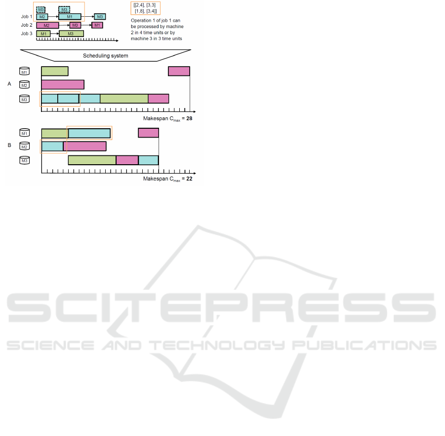
Figure 1: A comparison of two possible schedules demon-
strating the benefit of cooperative behavior between agents.
Three jobs colored in blue, red and green with three consec-
utive operations should be assigned to three machines. Job 1
(blue) has two options for operations one and two with dif-
ferent processing times (orange rectangle). In schedule A,
the faster options are chosen leading to a sub-optimal over-
all schedule. In schedule B, the slower options are chosen
for Job 1, allowing other agents to perform their operations
sooner, achieving a schedule that is 6 time units faster.
The first phase utilizes dense local rewards from (Baer
et al., 2020b) to ensure fast learning and simplified
credit assignment. Following this, the second phase
involves re-training with the local rewards augmented
by a global reward factor (see Section 4.3). The sec-
ond approach involves using a sparse global reward
during training, i.e. all agents receive a single reward
signal at the end of an episode (see Section 4.4). To
facilitate learning from a single reward signal, eligi-
bility traces (Sutton and Barto, 2012) are used instead
of experience replay.
We expect that the global reward approaches in
combination with the state design described in Sec-
tion 3.1 should enable the agents to learn when co-
operative actions might be necessary. As the state in-
cludes information not only about the product of the
agent but also about the products handled by other
agents, this should allow an agent to anticipate the ac-
tions of other agents to some extent and to adjust its
own actions for better cooperation.
4.3 Dense Reward Design
For the dense reward approach, the training is sep-
arated into two phases: “training” and “re-training”.
During the first training phase, only dense local re-
wards are used, as in (Baer et al., 2020b). In this
phase, the agents are supposed to learn a fundamental
behavior policy involving the understanding of which
actions are valid at which position as well as how
to interpret the job specification input, recognizing
which machines can be entered to process each op-
eration. Furthermore, the agents begin to learn to
achieve a local optimization, i.e. to minimize their
local makespan. During the re-training phase, the lo-
cal rewards are augmented by multiplying them with
a global reward factor that is calculated based on the
total makespan. This global reward factor adjusts the
dense rewards to a value that is either slightly larger,
in the event of a good total makespan, or slightly
smaller, in the event of a bad total makespan. This
is supposed to fine-tune the agents’ behavior with re-
spect to the global optimization goal.
Calculating a global reward is only viable when
all agents finish their jobs correctly and the total
makespan is known. During the first training phase,
the agents learn to recognize valid actions through un-
derstanding the job specification and the flexible pro-
duction system. Therefore, during re-training most
exploitative actions are ensured to be valid. In addi-
tion, it is implemented that the agents can only choose
exploratory actions that are valid given their current
location. In case an agent still chooses an invalid ac-
tion (through exploitation) and the episode is not com-
pleted, no global reward is calculated for the episode.
As the global reward is determined at the end of
the episode, the initial local rewards calculated dur-
ing the episode are changed retroactively in the re-
play memory. For this, the initial local rewards are
boosted by multiplying them with the global reward
factor calculated after the episode. Negative values
are not boosted with the global reward factor to avoid
excessive discouragement of exploration.
For determining the size of the global reward fac-
tor, it must be evaluated whether or not the generated
schedule is good with respect to the global optimiza-
tion goal, i.e. if the total makespan is close to the
optimum. However, during training, an optimal to-
tal makespan is not known, as an optimal schedule
cannot be calculated ad hoc (at least not for arbitrary
cases). Therefore, the optimal total makespan cannot
be used as a reference to calculate the global reward
factor. Furthermore, as we select a new random com-
bination of job specifications every n epochs (from
a fixed data set), it would be unreasonable to have
all necessary optimal schedules computed beforehand
and stored in a data set in which each job specification
combination is labeled by the optimal total makespan.
Whilst in the chosen use case such an approach could
be possible, the computation time may become pro-
hibitive in larger problem instances.
Therefore, to determine the global reward, an es-
Global Reward Design for Cooperative Agents to Achieve Flexible Production Control under Real-time Constraints
519

timated upper and lower bound is calculated in which
the total makespan of the schedule is most likely to be
found depending on the three job specifications used
in a certain episode of the training. In the first step,
an upper and lower bound is calculated for each job
specification individually. Figure 2 shows an example
of how the lower bound is calculated for three differ-
ent job specifications. As can be seen, the processing
time of each operation is added, assuming that each
time the machine with the lowest processing time is
selected. In addition, the transportation time between
the different machines is also calculated and added.
The transportation time is determined based on the
plant topology. The upper bound for each job spec-
ification is calculated in the same way with the only
difference being that, for each operation, the machine
with the highest processing time is selected.
Figure 2: Demonstration of the calculation of the lower
bound for three given job specifications.
After calculating the individual bounds for each job
specification, the global bounds are calculated using
b
LG
= max(b
L
( js
1
), b
L
( js
2
), b
L
( js
3
)) ∗ c
1
+ c
2
b
UG
= max(b
U
( js
1
), b
U
( js
2
), b
U
( js
3
)) ∗ c
3
+ c
4
(3)
where js
i
is equal to the job specification for agent i,
b
LG
and b
UG
are the global lower and upper bounds,
and b
L
and b
U
are the local lower and upper bounds of
each job respectively. The maximum lower bound is
selected as the global lower bound and the maximum
upper bound is selected as the global upper bound.
This is because all three agents together can only fin-
ish as quickly as the slowest agent.
It should be noted that these bounds are only an es-
timate and the actual makespan could be above or be-
low these thresholds. This is because when choosing
the best/worst machine for each operation neither the
transportation times are taken into account, nor is it
considered that agents may have to wait for resources.
To account for this, the empirical constants c
1
, ..., c
4
are introduced. Through an analysis of the generated
total makespans for a number of experiments during
training with respect to the calculated bounds, suit-
able values for the constants are determined to be
c
1
= 1, c
2
= c
4
= 0, c
3
= 1.1. This means that only
the upper bound is increased by ten percent which
seems reasonable to account for the agents blocking
resources for each other.
To finally calculate the global reward factor after
an episode given the global upper and lower bounds
of the job specifications used, various functions were
tested in advance. Figure 3 shows the function which
is used for the experiments in this paper, for an ex-
ample global lower bound of 30 and global upper
bound of 60. The label “Mean” indicates the mean
value between the two bounds. If the agents’ behav-
ior leads to a total makespan lower than the mean,
they receive a global reward factor higher than 1, in-
creasing the local rewards through multiplication. If
the total makespan is higher than the mean, the global
reward factor is lower than 1 decreasing the local re-
wards. However, the global reward decreases the local
reward by a maximum factor of 0.8.
Figure 3: Plot of the function which is used to map the total
makespan to a global reward factor given the global upper
and lower bound.
Formally, the global reward function R
glo
(t) is defined
as:
R
glo
=
3
m−t
m−b
LG
if t ≤ m
−
0.2
b
UG
−m
t +
0.2m
b
UG
−m
+ 1 if m < t ≤ b
UG
0.8 if t > b
UG
(4)
with b
UG
and b
LG
being the global upper and lower
bound for the job specifications, m being the mean
value, and t being the total makespan.
Determining this function required several itera-
tions of fine-tuning. While it initially seemed reason-
able to penalize the agents for schedules below the
mean with a global reward factor between 0 and 1,
this led to poor results. As the total makespan is of-
ten close to the upper bound during initial stages of
the training, the agent’s local reward for entering a
correct machine is almost completely eliminated due
to a global reward factor close to 0. As a result, in
some validation scenarios, the agents circled on the
ICEIS 2021 - 23rd International Conference on Enterprise Information Systems
520

conveyor belt without ever entering a machine as they
were discouraged by the low reward. Therefore, the
global reward function is adapted to never drop below
0.8. Furthermore, we also examined whether it pro-
vides any benefit to set an upper limit to the global
reward factor, as high global rewards may lead to a
large variation in the Q-values during training, ulti-
mately aggravating learning. However, it was shown
that setting an upper limit is not necessary as the lower
bound is rarely exceeded during training.
4.4 Sparse Reward Design
In contrast to the dense reward design described in
the previous section, we also explore the approach
of training the agents using a sparse global reward
in which all agents receive a common reward sig-
nal at the end of the episode depending on the total
makespan. Furthermore, the training is not separated
into two phases. Instead, the agents are trained us-
ing the sparse global reward right from the beginning.
While sparse rewards are usually much more intuitive
from the modeling standpoint, they might aggravate
learning in complex tasks. With regard to the exam-
ined scheduling domain, the agents might have trou-
ble learning a functioning policy if they are not ex-
plicitly rewarded for reaching subgoals such as pro-
cessing an operation by entering a correct machine.
Nevertheless, sparse rewards are commonly used in
many domains and often demonstrate remarkable re-
sults.
As no local rewards exist, the agents can only
learn from the sparse global reward. The sparse global
reward in turn requires all agents to finish their prod-
ucts correctly so that the total makespan is known.
Therefore it must be ensured from the beginning of
training that the agents can only choose valid actions.
For this, we apply Q-value masking similar to (Kool
et al., 2019) and (Bello et al., 2017). In Q-value mask-
ing, the action space of the agent is masked so that the
agent can only choose between valid actions. During
exploration one of the valid actions is selected ran-
domly and during exploitation the valid action with
the highest Q-value is selected. If an invalid action
has a higher Q-value, it is disregarded.
To keep the experiments between the two reward
designs as comparable as possible, the sparse global
reward is defined to resemble the previously used
dense local reward design (see eq. (2)). As the agents
received a local reward of +2 for entering a valid ma-
chine minus a penalty of −0.1 for every time step
spent in the machine (waiting or processing) as well
as a reward of −0.1 for every time step on the con-
veyor belt, and each job comprises four operations,
the sparse global reward is calculated as:
R
sparse
= 8 − (total makespan ∗ 0.1). (5)
To facilitate learning from a sparse reward signal,
we use eligibility traces (Sutton and Barto, 2012).
In comparison to regular Q-learning, in which the
action-value function is updated considering only the
state at time step t and the state at t + 1, eligibility
traces also take past states into account by extending
what has been learned at t + 1 also to previous states.
This accelerates learning as the action-value of the
first action in the episode is also affected by the up-
date of the last action-value, in which the only reward
is received. As eligibility traces require the process-
ing of the experiences in the same order as they occur
during an episode, experience replay cannot be used.
Therefore, we save entire trajectories of the agents in
a buffer. When an epoch is completed, all saved tra-
jectories are processed in sequential order while per-
forming the corresponding Q-value updates using eli-
gibility traces.
5 EXPERIMENTS
To find out whether the (re-)training with global re-
wards provides any benefits concerning a global op-
timization compared to training only with local re-
wards, several experiments are conducted. The hyper-
parameters that are used are mainly based on results
of the hyperparameter study conducted in (Baer et al.,
2020b). For the following experiments, the agents are
trained for 4,000 epochs. In the case of the dense re-
ward strategy, the epochs are split equally among the
two training phases, which means that the last 2,000
epochs are used for re-training with global rewards.
The Q-network comprises two (fully-connected) hid-
den layers with 128 and 64 nodes respectively, along-
side the input layer with 522 nodes and the output
layer with 24 nodes. The hidden layers use ReLU
activations while the output layer uses linear activa-
tion. Furthermore, we use a discount rate (gamma) of
0.95, a learning rate of 0.0001, and stochastic learn-
ing when performing the network updates. The re-
play memory size of each agent is 4,096 leading to a
common replay memory of 12,276. During each ex-
perience replay, we sample 8,192 experiences for up-
dating the Q-network. The training set contains 600
job specifications which are sampled in random order.
Every fifth epoch of training, the job specifications are
changed.
For the experiment using a sparse global reward,
we start with an epsilon value of 0.99 and decrease
the value over time using an epsilon decay of 0.9992.
Global Reward Design for Cooperative Agents to Achieve Flexible Production Control under Real-time Constraints
521

This leads to an exponential decrease with epsilon
reaching its defined minimum value of 0.05 after
around 90% of the training. For the experiment using
dense rewards, the epsilon development is adjusted to
account for the two training phases. The training also
starts with an epsilon value of 0.99. However, we use
an epsilon decay of 0.9984 so that the minimum of
0.05 is already reached after around 1,850 epochs.
Before the re-training starts after 2,000 epochs, the
epsilon value is reset to 0.9. This allows the agents to
explore again and adjust their behavior according to
the changed reward function during re-training.
For evaluating the experiments, we use ten scenar-
ios, in each of which three unseen products must be
scheduled by the agents. The validation set is con-
sistent across all experiments. We compare the per-
formance of the two global reward designs with the
baseline performance of (Baer et al., 2020b) using
local rewards only. To further benchmark our sys-
tem, we also compare the results with common search
and optimization algorithms using the Python pack-
age mlrose (Hayes, 2019). Namely, the algorithms
“hill climb”, “genetic algorithm” and “simulated an-
nealing” are tested (Russell and Norvig, 2009). As
simulated annealing consistently performed the best
among all optimization algorithms tested, we only ad-
dress those results in Section 6.
As our scheduling task is a discrete-state opti-
mization problem, we apply the aforementioned algo-
rithms of mlrose to the corresponding problem class
(mlrose.DiscreteOpt). In addition, we define a custom
fitness function (mlrose.CustomFitness) which corre-
sponds to the total makespan of a schedule. The opti-
mization algorithms try to find a suitable array of re-
source allocations that minimizes the defined fitness
function. The array defines which operation of which
job should be processed by which machine. Since the
jobs in each validation scenario have four operations,
the array contains 12 values. Each value is ranged
between 1 and 6, as there are six machines available,
leading to 6
12
possible different states. The custom
fitness function calculates the total makespan for a
given state. It considers the transportation time be-
tween the machines using a distance matrix as well as
resource blockades so that the results are comparable
to the RL system. For invalid states, i.e. states that do
not fulfill the job specifications, additional penalties
to the fitness function lead to a return value higher
than the total makespan of any valid schedule. Pa-
rameters defining the maximum number of iterations
or the maximum number of attempts of the algorithms
are set to values that lead to a run-time of around 15
minutes on a modern server CPU. It was shown that
higher numbers of iterations do not lead to better re-
sults in most cases.
6 RESULTS
6.1 Global Optimization
Table 1 shows a comprehensive analysis of the exper-
iments. Each row in the table corresponds to one of
the validation scenarios in which three unseen jobs
are scheduled. The values indicate the total makespan
achieved for each scenario. Furthermore, the valida-
tion is done with the network weights after 2,000 and
4,000 epochs of training. In the case of training with
dense rewards, this is necessary to find out whether re-
training with global rewards had a positive effect on
the agents’ behavior concerning the total makespan.
Furthermore, to rule out that any improvement is due
to the additional 2,000 epochs of training and not to
the global reward design, the table also shows the re-
sults after re-training with local rewards only.
The four columns on the left of Table 1 show
the results of the dense reward approach. As can
be seen in the first two columns, the continued train-
ing with dense local rewards did not lead to any im-
provement. The policy marginally changed during
re-training leading to some validation scenarios be-
ing scheduled slightly better and some slightly worse.
However, the average total makespan for the valida-
tion scenarios overall stayed the same. The third col-
umn shows the results after re-training with the dense
local rewards being boosted by a global reward fac-
tor. Analyzing the average total makespan shows a
significant improvement of around 10% compared to
the baseline. In three validation scenarios, the total
makespan became slightly worse, in one scenario it
stayed the same, and in six of the validation scenar-
ios, the total makespan was improved by up to 25%.
This confirms the effectiveness of including a global
reward component during re-training with respect to
achieving a smaller total makespan.
The middle section of Table 1 shows the results of
using a sparse global reward. It can be seen that af-
ter training for 4,000 epochs, a similar performance is
achieved for the validation scenarios compared to the
dense global reward variant. As in this case, the train-
ing is not separated into two phases, the validation
after 2,000 and 4,000 epochs does not demonstrate
the benefit of re-training with a global reward compo-
nent, but simply shows the progress after additional
training.
Although the usage of a sparse global reward did
not lead to an improvement over the dense reward de-
sign, it is still remarkable how well the agents are able
ICEIS 2021 - 23rd International Conference on Enterprise Information Systems
522
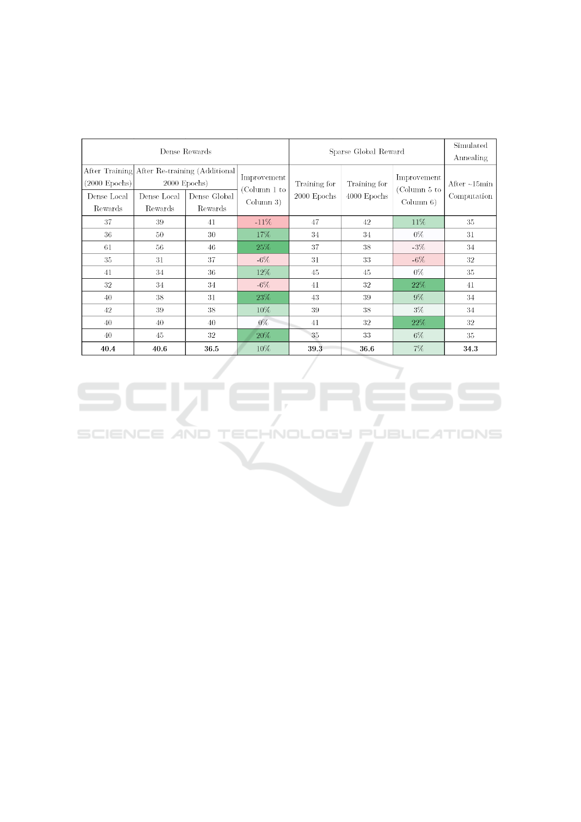
Table 1: Comprehensive analysis of the agents’ performance with respect to the total makespan after being (re-)trained using
the described global reward variants. Both implemented global reward designs led to a significant improvement compared to
the baseline using local rewards only. The comparison with simulated annealing shows that there is still room for improve-
ment.
to learn from a single reward signal at the end of the
episode. This is an important realization, as imple-
menting the sparse reward design required much less
effort compared to the dense reward design. The im-
plementation of functioning dense local rewards and
the augmentation of these rewards with elaborately
calculated global reward factors required much more
engineering effort and fine-tuning than the sparse re-
ward design. The fact that the sparse reward is calcu-
lated solely based on the total makespan and does not
require the comparison to any hypothetical bounds (as
done in the dense reward design) makes the imple-
mentation much easier and more universally applica-
ble.
To rule out the possibility that the good perfor-
mance of the sparse reward design is coming from
the use of Q-value masking and not from the re-
ward design itself, a number of experiments with the
dense reward design are repeated while also using Q-
value masking. The results have demonstrated a clear
drop in performance when Q-value masking is en-
abled. This confirms that making invalid actions dur-
ing training and receiving an instant negative reward
for it substantially helps the agents to learn. Train-
ing schemes involving the sparse global reward with-
out Q-value masking, on the contrary, hardly allow
the agents to learn at the initial training stage as very
few episodes are completed successfully without the
agents making invalid actions. Therefore, while Q-
value masking remains an important part of the train-
ing process involving the sparse global reward, it can
be seen as a necessary but insufficient condition for
good results.
The comparison to simulated annealing is shown
in the rightmost column of Table 1. The average to-
tal makespan for the tested scheduling scenarios us-
ing simulated annealing is slightly better compared
to the performance achieved by the RL system after
being trained with one of the global reward variants.
However, it can also be seen that in some of the val-
idation scenarios, the total makespan of the schedule
generated by the RL system is even better than the
one found by simulated annealing. While this com-
parison shows that there is still room for improve-
ment regarding the total makespan, the performance
of the RL system is already very promising and suit-
able for practical application. Furthermore, it should
be stressed that the RL system is designed to be used
for online scheduling, meaning that the focus lies less
on optimality but more on reactivity and real-time
decision-making. The RL system has the advantage
of being able to react instantly to changes during pro-
duction as each new decision only requires a single
forward pass of the trained network. For example,
if an additional manufacturing skill is activated on a
machine during production, the agent would receive
this information through a changed job specification.
The agent sees in its job specification lookahead for
Global Reward Design for Cooperative Agents to Achieve Flexible Production Control under Real-time Constraints
523

its next operation which machines are available and
can act accordingly. Using an offline scheduling ap-
proach (as demonstrated with simulated annealing), a
completely new scheduling plan would have to be cal-
culated if a slight change occurs during production.
This would require several minutes, leading to idle
time in the production, and, therefore, would not be
suitable for reactive production control fulfilling the
given requirements.
Regarding the tested validation scenarios, simu-
lated annealing achieved about equal performance to
the RL system after around five minutes of compu-
tation and converged after around 15 minutes to the
results displayed in the table. The RL system on the
contrary requires much less time and can react in real-
time, as only a few inferences of the (small) trained
network are required.
Figure 4 summarizes the experimental results. By
looking at the spread and median makespan values
achieved by the trained agents on the set of valida-
tion scenarios it can be derived which reward designs
facilitate the learning of good scheduling heuristics.
The lower the median value and spread of the ob-
served makespan values are, the better the schedul-
ing heuristic learned by the agent. Dense local re-
wards provide the agents with a rich signal enabling
fast learning during the first 2,000 epochs. How-
ever, since no global minimization of the makespan
can be embedded into the local reward design, fur-
ther training for 2,000 epochs does not result in any
better performance. Sparse global rewards, on the
contrary, provide a learning signal directly tailored
to the minimization of the total makespan. Agents
trained with the sparse global reward do not show any
learning advantage over the dense local reward de-
sign during the first 2,000 epochs. However, contin-
uing training for another 2,000 epochs significantly
improves the learned behavior both in terms of the
makespan median values and the spread across the
different scheduling scenarios. However, the quality
of the learned behavior based only on the sparse re-
ward might quickly decay with scheduling tasks of
growing size. Longer planning horizons aggravate
the challenge of credit assignment to single good ac-
tions over long episodes. Agents jointly trained on
dense local rewards and global rewards can incorpo-
rate the best of both by using a rich learning signal
tailored to the global optimization goal. In our exper-
iments, agents trained on the combination of dense
local and global rewards achieve a comparable me-
dian makespan to the agents trained solely on a sparse
global reward. While surpassing all other reward ap-
proaches and simulated annealing by a good margin
in some of the scheduling instances, it has an overall
Local Rewards (2000 Epochs)
Local Rewards (4000 Epochs)
Sparse Global Rewards (2000 Epochs)
Sparse Global Rewards (4000 Epochs)
Local and Global Rewards (4000 Epochs)
Simulated Annealing
30
35
40
45
50
55
60
Solution Approach
Makespan
Figure 4: Comparative analysis of different RL training
strategies and simulated annealing.
higher variance compared to the agents trained with
the sparse global reward for 4,000 epochs. The per-
formance of simulated annealing is 6% better on av-
erage compared to the best RL agents at the cost of
considerably longer computation time.
6.2 Cooperative behavior
In the previous section, it has been shown that the
agents have managed to improve the total makespan
on the validation scenarios after being trained using
one of the global reward strategies. However, it is
unclear whether this improvement is achieved by the
agents collaborating or simply by each agent making
better decisions for itself. Therefore, the schedules
of the validation scenarios are analyzed to find out
whether the agents have actually developed any ten-
dency toward cooperative behavior. For this, we use
the Gantt charts created during the evaluation of the
dense global reward design after 4,000 epochs, as this
had the best overall performance.
The analysis has shown that in some of the cases
with reduced total makespan after re-training, the im-
provement is achieved by the agents finding better in-
dividual schedules and do not necessarily involve co-
operation. However, this can be due to the fact that
some job specification combinations used for vali-
dation simply did not have any conflicting schedul-
ing situations that require cooperation for achieving a
(near-)optimal total makespan. In other cases, the im-
provement could be attributed to cooperative actions
in which an agent degraded its individual performance
but improved the performance of other agents.
To further examine the cooperativeness, additional
validation scenarios are manually created with special
emphasis on job specifications that require collabora-
tion. The analysis of these schedules has confirmed
that the agents do in fact cooperate in many cases
where necessary. Figure 5 shows one of these valida-
tion scenarios with the corresponding schedule before
ICEIS 2021 - 23rd International Conference on Enterprise Information Systems
524
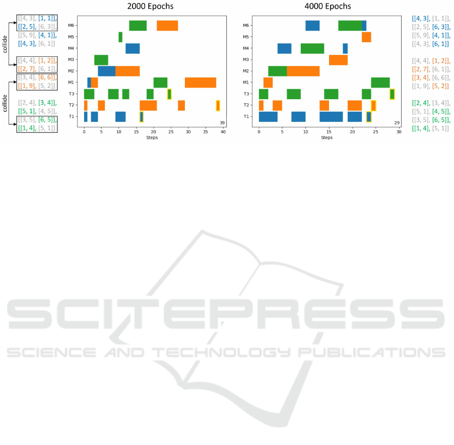
Figure 5: Comparison of two schedules with respect to the cooperativeness of the agents. After re-training (right), the agents
find a schedule with a much lower total makespan. While the different agents often chose the same machine for processing
an operation after 2,000 epochs (left), they have learned after re-training to spread more equally across the different machine
options and, hence, avoid unnecessary waiting times.
and after re-training with the global reward. The job
specifications are designed so that the first two opera-
tions of the first and second job collide, as well as the
second two operations of the second and third job.
Figure 5 shows that the agents have learned dur-
ing re-training to choose a worse option if it allows
another agent to be faster and therefore improves the
overall total makespan. For example, after train-
ing with local rewards (2,000 epochs), both Agent 1
(blue) and Agent 2 (orange) choose M1 for the first
operation and M2 for the second operation, causing an
unnecessary queue. However, after re-training, Agent
1 instead chooses M4 and M6, which is worse locally,
but allows Agent 2 to finish almost 15 time steps ear-
lier. Agent 3 (green) also chooses M2 for its first op-
eration, although this causes a queue, as the overall
makespan is still better this way. Furthermore, for the
third and fourth operation, Agent 2 and Agent 3 ini-
tially both chose M6 and M1 respectively. However,
after re-training with global rewards, Agent 2 chooses
M3 and M5 to avoid collisions (although this is also
the better option locally for this case).
7 CONCLUSION
In this paper, we have presented two global reward
designs for enabling cooperative behavior between
multiple agents in a flexible manufacturing system.
The proposed multi-agent system is capable of solv-
ing scheduling tasks with the global optimization goal
of minimizing the total makespan. The first reward
design uses dense local rewards in an initial training
phase and augments the local rewards by a global re-
ward factor during a re-training phase. The second
approach uses a sparse global reward depending on
the achieved total makespan. To facilitate learning
from the sparse reward, eligibility traces and Q-value
masking are used.
Both global reward designs demonstrate signif-
icantly better results in terms of the achieved total
makespans compared to the baseline solution of (Baer
et al., 2020b) training with local rewards only. We
observe an improvement of 10% of the average to-
tal makespan by augmenting the dense local rewards
with a global reward factor. Comparable results are
achieved by the sparse global reward design while re-
quiring much less engineering effort. A detailed anal-
ysis of the Gantt charts generated for the validation
instances has also confirmed the positive influence of
global rewards in regards to the cooperative behavior
of the agents. After being trained with local rewards,
it could be observed that the agents mostly act self-
ishly and fail to generate schedules with a low total
makespan. However, after using one of the proposed
global reward variants, the agents were shown to co-
operate in most cases by selecting actions with neg-
ative influence on their own local performance, but a
positive effect on the global optimization goal.
Among the tested non-learning-based heuristics,
simulated annealing delivers on average a 6% better
makespan after around 15 minutes of computation.
Equal performance to our RL system is achieved af-
ter 5 minutes. However, the RL system finds suit-
able schedules within seconds as each decision only
requires the inference of a small neural network. This
makes our solution particularly viable for applications
in flexible and reactive scheduling.
Despite the promising results achieved in this pa-
per, the RL system still has some limitations that
should be addressed in the future for use in practi-
cal applications. For example, it would be interesting
to consider more than three products in the system
at the same time. This would further emphasize the
Global Reward Design for Cooperative Agents to Achieve Flexible Production Control under Real-time Constraints
525

necessity for cooperation and also require the selec-
tion of relevant information about the other agents for
the local state. In addition, it would be worthwhile to
allow products to enter the system dynamically over
time, which would require the re-definition of the op-
timization goal for training (e.g. using throughput in-
stead of makespan). Another direction of future work
would be to extend the system to be able to handle
open-shop scheduling problems, in which the opera-
tions of a job do not necessarily have to be processed
in a fixed order. Furthermore, it should be investigated
how agents trained in the discrete simulation behave
in a real manufacturing system, which is much more
dynamic, and to which extent re-training of the net-
work is needed.
REFERENCES
Baer, S., Baer, F., Turner, D., Pol, S., and Meisen, T.
(2020a). Integration of a reactive scheduling solution
using reinforcement learning in a manfacturing sys-
tem. In Automation 2020, Bade-Baden, Germany.
Baer, S., Turner, D., Kumar Mohanty, P., Samsonov, V.,
Bakakeu, R. J., and Meisen, T. (2020b). Multi agent
deep q-network approach for online job shop schedul-
ing in flexible manufacturing. In ICMSMM 2020: In-
ternational Conference on Manufacturing System and
Multiple Machines, Tokyo, Japan.
Bello, I., Pham, H., Le, Q. V., Norouzi, M., and Bengio, S.
(2017). Neural combinatorial optimization with rein-
forcement learning.
Bernstein, D., Givan, R., Immerman, N., and Zilberstein,
S. (2002). The complexity of decentralized control of
markov decision processes. Mathematics of Opera-
tions Research, 27.
Berrada, M. and Stecke, K. E. (1986). A branch and
bound approach for machine load balancing in flex-
ible manufacturing systems. Management Science,
32(10):1316–1335.
Cs
´
aji, B. C. and Monostori, L. (2004). Adaptive algorithms
in distributed resource allocation. In Proceedings of
the 6th International Workshop on Emergent Synthesis
(IWES 2004), pages 69–75.
De Hauwere, Y.-M., Vrancx, P., and Nowe, A. (2010).
Learning multi-agent state space representations. In
Proceedings of the International Joint Conference on
Autonomous Agents and Multiagent Systems, AAMAS,
volume 2, pages 715–722.
Foerster, J., Assael, I. A., de Freitas, N., and White-
son, S. (2016). Learning to communicate with deep
multi-agent reinforcement learning. In Lee, D. D.,
Sugiyama, M., Luxburg, U. V., Guyon, I., and Garnett,
R., editors, Advances in Neural Information Process-
ing Systems 29, pages 2137–2145. Curran Associates,
Inc.
Gabel, T. and Riedmiller, M. (2007). Scaling adaptive
agent-based reactive job-shop scheduling to large-
scale problems. In 2007 IEEE Symposium on Com-
putational Intelligence in Scheduling, pages 259–266.
Garey, M. R., Johnson, D. S., and Sethi, R. (1976).
The complexity of flowshop and jobshop scheduling.
Mathematics of operations research, 1(2):117–129.
Gupta, J. K., Egorov, M., and Kochenderfer, M. (2017).
Cooperative multi-agent control using deep reinforce-
ment learning. In Sukthankar, G. and Rodriguez-
Aguilar, J. A., editors, Autonomous Agents and Multi-
agent Systems, pages 66–83, Cham. Springer Interna-
tional Publishing.
Hayes, G. (2019). mlrose: Machine Learning, Random-
ized Optimization and SEarch package for Python.
https://github.com/gkhayes/mlrose.
Kool, W., van Hoof, H., and Welling, M. (2019). Attention,
learn to solve routing problems!
Kuhnle, A., Kaiser, J.-P., Theiß, F., Stricker, N., and Lanza,
G. (2020). Designing an adaptive production control
system using reinforcement learning. Journal of Intel-
ligent Manufacturing.
Manne, A. S. (1960). On the job-shop scheduling problem.
Operations Research, 8(2):219–223.
Mnih, V., Kavukcuoglu, K., Silver, D., Graves, A.,
Antonoglou, I., Wierstra, D., and Riedmiller, M.
(2013). Playing atari with deep reinforcement learn-
ing.
Panait, L. and Luke, S. (2005). Cooperative multi-agent
learning: The state of the art. Autonomous Agents and
Multi-Agent Systems, 11(3):387–434.
Roesch, M., Linder, C., Bruckdorfer, C., Hohmann, A., and
Reinhart, G. (2019). Industrial load management us-
ing multi-agent reinforcement learning for reschedul-
ing. In Second International Conference on Artificial
Intelligence for Industries (AI4I), pages 99–102.
Russell, S. and Norvig, P. (2009). Artificial Intelligence:
A Modern Approach. Prentice Hall Press, USA, 3rd
edition.
Sukhbaatar, S., Szlam, A., and Fergus, R. (2016). Learning
multiagent communication with backpropagation. In
Lee, D. D., Sugiyama, M., Luxburg, U. V., Guyon, I.,
and Garnett, R., editors, Advances in Neural Informa-
tion Processing Systems 29, pages 2244–2252. Curran
Associates, Inc.
Sutton, R. S. and Barto, A. G. (2012). Reinforcement learn-
ing: An introduction. A Bradford book. The MIT
Press, Cambridge, Massachusetts.
Waschneck, B., Reichstaller, A., Belzner, L., Altenm
¨
uller,
T., Bauernhansl, T., Knapp, A., and Kyek, A. (2018).
Deep reinforcement learning for semiconductor pro-
duction scheduling. In 2018 29th annual SEMI
advanced semiconductor manufacturing conference
(ASMC), pages 301–306. IEEE.
ICEIS 2021 - 23rd International Conference on Enterprise Information Systems
526
