A Full-Featured, Enhanced Cost Function to Mitigate Motion

Sickness in Semi- and Fully-autonomous Vehicles

Isa Moazen and Paolo Burgio

HiPeRT Lab., University of Modena and Reggio Emilia, Italy

Keywords: Motion Sickness, Autonomous Driving, Comfort, Model-Predictive Control, Cost-function, Embedded

Control Systems.

Abstract: Current full- and semi- Autonomous car prototypes increasingly feature complex algorithms for lateral and

longitudinal control of the vehicle. Unfortunately, in some cases, they might cause fussy and unwanted effects

on the human body, such as motion sickness, ultimately harnessing passengers' comfort, and driving

experience. Motion sickness is due to conflict between visual and vestibular inputs, and in the worst case

might causes loss of control over one’s movements, and reduced ability to anticipate the direction of

movement. In this paper, we focus on the five main physical characteristics that affect motion sickness,

including them in the function cost, to provide quality passengers' experience to vehicle passengers. We

implemented our approach in a state-of-the-art Model Predictive Controller, to be used in a real Autonomous

Vehicle. Preliminary tests using the Unreal Engine simulator have already shown that our approach is viable

and effective, and we implemented and evaluated using Motion Sickness Dose Value and Illness Rating and

then tested it in an embedded platform. We implemented it on our embedded platform, NVIDIA Jetson AGX

Xavier that is representative of the next-generation AV Domain Controller.

1 INTRODUCTION

In semi- and full AVs, vehicle control shall consider

passengers’ stress, and not decrease their level of

comfort (Elsner, 2018). It was proven that a tight

relationship exists between comfort and trust, as well

as the acceptance of automated vehicles (Bellem et

al., 2018).

The mostly known comfort issues for the

passengers is probably Motion Sickness. Its common

symptoms are: headache, pallor, sweating, nausea,

vomiting, and disorientation, and they can be

measured by Physiological signals, Vestibule Ocular

Reflex (VOR) parameters, and Posture stability.

There are several ways to mitigate this, such as

instance visual cues, Posture and vehicle

controllability, and Immersive Experience (Iskander

et al., 2019).

Motion is primarily sensed by the organs of

balance located in the inner ear and our eyes, which

are mainly or uniquely sensitive to accelerations. The

vestibular section of the inner ear is partly comprised

of three semi-circular canals that detect head angular

acceleration. The main issue stems from the fact that

our bodies are not used to low-frequency oscillating

motion, and our “biological IMUs” are highly

sensitive to this. In carsickness, the lateral

accelerations (sway) in the low-frequency bands (0.1-

0.5 Hz) are most relevant and their effects increase in

higher accelerations. In general, researchers proved

(Diels, 2014) that it might happen when the frequency

is below 1 Hz.

The potential sources of AV motion sickness are

variation in horizontal and vertical acceleration,

posture instability, loss of controllability and loss of

anticipation of motion direction, Head downward

inclination, and lack of synchronization between

virtual motion and the vehicle motion profile

(Iskander et al., 2019). Although motion sickness is

most frequently caused by a conflict between visual

and vestibular inputs, loss of control over one’s

movements and reduced ability to anticipate the

direction of movement are also important in the

etiology of motion sickness (Sivak and Schoettle,

2015). All three factors, to varying degrees, are more

frequently experienced by vehicle passengers than by

drivers, who rarely experience motion sickness

(Sivak and Schoettle, 2015). Possible counter

measures can be categorized into two groups:

prevention solutions and mitigation solutions.

Moazen, I. and Burgio, P.

A Full-Featured, Enhanced Cost Function to Mitigate Motion Sickness in Semi- and Fully-autonomous Vehicles.

DOI: 10.5220/0010446604970504

In Proceedings of the 7th International Conference on Vehicle Technology and Intelligent Transport Systems (VEHITS 2021), pages 497-504

ISBN: 978-989-758-513-5

497

Roughly speaking, the degree of motion sickness may

be predicted by an acceleration frequency weighting

that is independent of frequency from 0.0315 to 0.25

Hz and reduces at 12 dB per octave (i.e., proportional

to displacement) in the range 0.25 to 0.8 Hz (Iskander

et al.., 2019).

We contribute to research with the original design

of a control software component for AVs that

minimizes the most important costs. In this paper, we

used an Adaptive Model Predictive Control (AMPC)

that can estimate and update the model in real-time

along with five constraints to build our cost function

to minimize.

We have chosen the constraints that are relevant

to Motion Sickness and comfort, either direct or

indirect. Acceleration frequency is one of the

constraints that directly affects the Motion Sickness

and the range of Frequency in which Motion Sickness

occurs is in 0.0315<F<0.8 Hz (Donohew & Griffin,

2004). Speed limitation is not directly related to

Motion Sickness level. However, as the speed goes

up, Acceleration Frequency for the speed regulation

will arise. Therefore, we consider a speed limitation

based on our Acceleration Frequency. The European

New Car Assessment Program (Euro NCAP)

performed standardizing tests on different

autonomous vehicles with a constant speed of 20 – 60

km/h (Standard, 1987). We also consider a threshold

of acceleration because it affects both Motion

Sickness and Comfort driving (Standard, 1987). It is

also one of the factors that increase Motion Sickness

Dose Value (MSDV). Therefore, having the

limitation with an appropriate planner can lower the

MSDV and raise comfort. We also consider the

distance from the next vehicle to brake with a

minimum acceleration, as we discussed before. In

particular, with higher distance from the next vehicle,

we require a lower braking acceleration. Finally,

since the lateral acceleration is the other important

source in MSDV (Donohew & Griffin, 2004), we

need a lane keeper to reduce our lateral accelerations

to a minimum quantity.

The system is tested on MATLAB/Simulink

(MATLAB, 2020) and then implemented on an

NVIDIA Xavier AGX. We evaluate our work based

on ISO 2631-1 (Standard, 1987) which a measure of

the probability of nausea that is called motion

sickness dose value (MSDV) and a simple linear

approximation between MSDV and mean passenger

named illness rating (IR) are considered as the

evaluation methods.

In the following sections, we first review the state-

of-the-art in motion sickness and MPC controller.

Then we describe the details of our controller.

Finally, we show our implementation, and discuss

experimental results with respect to the reference

metrics of motion sickness.

2 MOTION SICKNESS IN AV

LITERATURE

Several works are done for the motion sickness

mitigation and minimization in the recent years. In

(Elsner, 2018) a library of cost functions, consisting

of progress, comfort, and safety costs, is used to

evaluate the strategies generated by the three modules

distance keeper, lane selector, and merge planner. In

(Sivak & Schoettle, 2015), two strategies for reducing

the visual-vestibular conflict while watching videos

are investigated. One approach imposes visual stimuli

on or around the video screen to mimic the perceived

motion and forces of the moving vehicle. The other

method involves controlling the position of displayed

images in synchronization with vehicle motions and

passenger's head motions produced by vehicle

acceleration/deceleration, thus providing a video that

appears to be stabilized in relation to the movement

of the vehicle. In (Lambert et al., 2019), a method is

proposed for generating optimal Path Planning with

Clothoid Curves for passenger comfort, and their cost

is based on the squared distance along the curve,

made up of the first clothoid length, the second

clothoid length, and the straight line to the goal at the

end. An application of Motion Planning is presented

in (Htike et al., 2020) in order to minimize MSDV in

self-driving vehicles. Most of the works are

considering some parameters but not all to minimize.

However, since the Motion Sickness occurs based on

different sources, to minimize it, we need to consider

all of the Motion Sickness sources. In this manner, we

require to distinguish the actual direct and indirect

sources and try to minimize or remove them.

Furthermore, it is essential to consider comfort

driving while minimizing the Motions Sickness rate.

To overcome these important factors, as opposite to

the other works, our work considers the direct and

indirect sources of Motion Sickness and tries to

minimize them all in a single cost function to enhance

passengers’ comfort.

Considering recent AMPC implementations in

autonomous driving, concentrating on their cost

functions, there are several efforts. In (Easa &

Diachuk, 2020), an adaptive model predictive control

with three constraints, Lane Change-Related

Constraint, Location in Opposite Lane Constraint,

and Maneuver Completion, is applied for tracking the

VEHITS 2021 - 7th International Conference on Vehicle Technology and Intelligent Transport Systems

498

references being generated for the Autonomous

Vehicles on Two-Lane Highways. In (Shi et al.,

2020), they constructed an adaptive model predictive

control trajectory tracking system with the four

constraints. In (Wu et al., 2020), an adaptive model

predictive control (AMPC) scheme is developed to

improve the yaw stability for four-wheel-

independently actuated electric vehicles by

minimizing the total longitudinal forces of all wheels.

In (Luan et al., 2020), the side slip angle of the centre

of mass and the side slip angle of the tire as hard

constraints and the lateral acceleration as a soft

constraint are considered to propose an Adaptive

Model Predictive Control for Uncertain model

(UMAMPC) algorithm to predict control variables

for the next sampling time and alleviate the target

angle discontinuity. In (Geng and Liu, 2020), they

develop a fault tolerant path tracking control

algorithm through combining the adaptive model

predictive control algorithm for lateral path tracking

control and Kalman filtering approach with two states

chi-square detector and residual chi-square detector

for detection and identification of sensor fault in

autonomous vehicles by using the incremental

constraint of tire and the incremental constraint of

lateral acceleration.

In all of the above works, that are proposed for

controlling the autonomous vehicles by AMPC,

below than five constraints are used. In this work, we

use five constraints in an AMPC that minimize the

MSDV with consideration of comfort.

3 CONTROL SYSTEM

To design the controller, we defined a Vehicle Model

and used the tire forces to specify our state space.

Then, we entered our state space in AMPC and

defined our constraints in it.

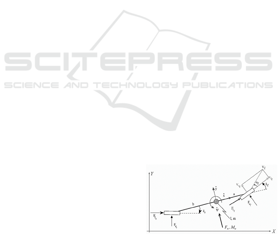
3.1 Vehicle Model

For an MPC control design, we require to define our

Vehicle Model. It was found that the vehicle side slip

angle is less than 1◦ in the highway autonomous or

manoeuvre driving under clothoid constraints (Kang

et al., 2014). Thus, it is considered that the tire slip

angle is also negligible under highway driving

conditions, including cases employing an advanced

driver assistant system (ADAS). It makes it possible

to use a standard dynamic “bicycle model”

(Rajamani, 2011) to describe the Vehicle Dynamics.

Such as a recent work (Antonelli et al., 2019) that uses

the higher speed until 35 m/s (126 km/h) with a

bicycle dynamic model, we use a bicycle dynamic

model for our tests between the speed of 0 km/h to 80

km/h and we use them in our first scenario. In the

bicycle model, the two left and right wheels are

represented by one single wheel. The model is

derived assuming both front and rear wheels can be

steered by δf and δr angles and the distances of front

and rear wheels are a and b. The model neglects roll

and pitch motions. The Motion of the vehicle is

represented by X, Y and ψ. Figure 1 depicts a diagram

of the vehicle model, which has the following

longitudinal, lateral, and turning or yaw equations:

𝑚𝑥 𝑚𝑟𝑦 𝐹𝑥



𝐹𝑥



(1)

𝑚𝑦 𝑚𝑟𝑥𝜓



𝐹𝑦



𝐹𝑦



(2)

𝐼



𝜓



𝑎𝐹



𝑏𝐹



(3)

The vehicle’s equations of motion in an absolute

inertial frame are

𝑌



𝑥sin𝜓 𝑦cos𝜓 (4)

𝑋



𝑥cos𝜓  𝑦sin𝜓 (5)

Longitudinal and lateral tire forces lead to the

following forces acting on the centre of gravity:

Fy = Fl sin δ + Fc cos δ, (6)

Fx = Fl cos δ − Fc sin δ. (7)

Tire forces for each tire are

Fl = fl(α, s, μ, Fz), (8)

Fc = fc(α, s, μ, Fz), (9)

where α is the slip angle of the tire and s is the slip

ratio. The tire model is considered as indicated in

(Filip, 2018) velocities, respectively, are expressed as

vl = vy sin δ + vx cos δ, (10)

vc = vy cos δ − vx sin δ, (11)

and

= ẏ + aψ



= ẏ − bψ



, (12)

= ẋ v

= ẋ. (13)

Figure 1: Bicycle Model of the Vehicle.

A Full-Featured, Enhanced Cost Function to Mitigate Motion Sickness in Semi- and Fully-autonomous Vehicles

499

If we consider δr =0, then:

𝑥 𝑟y 

 



(14)

ÿ𝑟y 

  



(15)

𝑟͘

 



(16)

Using the equations (1)-(16), the nonlinear

vehicle dynamics will have the states of



𝑋



𝑌



𝑣𝑥𝑣𝑦𝑟



3.2 Adaptive Model Predictive Control

System

MPC (Muske & Rawling, 1993) is a method for

process control that actively uses the dynamic model

of the system. If the nonlinearity is high, however,

MPC performance could deteriorate. In this case, one

can use an AMPC that constantly predicts the new

operating conditions. (Önkol and Kasnakoğlu, 2018).

An adaptive MPC algorithm is designed by using

the recursively-identified state-space models with

dynamic adjustments of MPC constraints and

objective function weights (Hajizadeh et al., 2020).

Adaptive MPC controllers adjust their prediction

model at run time to compensate for nonlinear or

time-varying plant characteristics. Furthermore,

Adaptive control for constrained systems has mainly

focused on improving performance with the adapted

models, while the constraints are satisfied robustly for

all possible model realizations and the worst

disturbance bounds (Aswani et al., 2013). In this

paper, we used an Adaptive MPC to update our state-

space online and get the linear part of our nonlinear

system. This approach is implemented with the most

important costs that we wanted to control.

In AMPC, the controller uses the time-varying

Kalman filter (TVKF) instead of the static one to

provide consistent estimation with the updated plant

dynamics. The TVKF approach can be expressed as

follows

𝐿



 𝐴



𝑃

|

𝐶

,



 𝑁𝐶

,

𝑃

|

𝐶

,



 𝑅



𝑀



 𝑃

|

𝐶

,



𝐶

,

𝑃

|

𝐶

,



 𝑅



(17)

𝑃

|

 𝐴



𝑃

|

𝐴





𝐴



𝑃

|

𝐶

,



 𝑁𝐿





 𝑄

In equation (17), Q, R, and N matrices are

constant covariance matrices, and Ak and Cm, k are

matrices depicting the state-space description of the

system. The Pk|k−1 is the state estimate error

covariance matrix at k constructed from the

information from time k−1. TVKF is constructed to

update regularly the L and M matrices with the

updated plant dynamics.

3.2.1 Constraints

The Model Predictive Control can directly include

constraints in the computation of the control moves

which leads to linear program (LP) or quadratic

program (QP) to be solved at each sampling instance,

with the constraints written directly as constraints in

the LP/QP.

The MPC algorithm solves a quadratic

optimization problem at each time interval. The

solution of the problem determines the so-called

manipulated variables (MV), which are essentially

the input variables adjusted dynamically to keep the

controlled variables (CV) at their set-points. The

AMPC approach follows the same cost optimization

algorithm as MPC with the cost function

𝐽





𝑧







∑∑





,









𝑟





𝑘𝑖

𝑘



𝑦



𝑘 𝑖|𝑘













(18)

where k represents the current control interval, p

is the prediction horizon (interval number), 𝑛



is the

number of plant output variables, 𝑧



is the quadratic

problem (QP) selection which is depicted as the

formula 𝑧





𝑢



𝑘|𝑘





𝑢



𝑘1|𝑘





…𝑢



𝑘𝑝

1|𝑘





𝑘, 𝑦





𝑘𝑖

𝑘



is the jth CV at the ith

prediction horizon step, 𝑟





𝑘𝑖

𝑘



is the ith

references variable at the ith prediction horizon step,

𝑠





is the scale factor for the jth plant output variable,

and 𝑤

,



is the tuning weight coefficient reflecting the

relative importance of the plant output variable.

Among these variables 𝑛



, 𝑠





, p, and 𝑤

,



, are

determined during the controller design and stay

constant.

Acceleration Frequency. The range of Frequency in

which Motion Sickness is tested in 0.0315<F<0.8 Hz.

However, the maximum Motion sickness occurs at

0.2 Hz (Donohew & Griffin, 2004). So we fixed

frequency at 0.2 Hz which means T= 5 s. In particular,

that we prevent inserting acceleration every 5

seconds.

Speed Limit. As discussed, the test speed is in the

range of 20 – 60 km/h (Standard, 1987). Since we

need to consider having acceleration and braking in

our work, we raised this limitation to 0 - 80 km/h and

in our tests, we consider these values.

Acceleration Limit. Acceleration limitation is an

important source for comfort and the different level

of comfort is measured based on it (Standard, 1987).

VEHITS 2021 - 7th International Conference on Vehicle Technology and Intelligent Transport Systems

500

Based on ISO 2631 (Standard, 1987) for

determination of acceleration, the best range of the

acceleration is <0.315 m/s2 that is named not

uncomfortable. In this standard, the best range of

acceleration is <1 m/s2 that is fairly uncomfortable

and it is the border of the uncomfortable range of

measurements. So we maintain this range.

Distance to the Front Vehicle. With a higher

distance from the next vehicle, we decrease the

braking acceleration. It means that we will have more

time to plan smooth braking, with the consideration

of our acceleration limit, and it lowers the MSDV.

There is a Two-Second Distance rule from the next

vehicle (Road Safety Authority, 2011). The mean

deceleration is 2.5 m/s2 (Yimer et al., 2020) and our

deceleration should not exceed 1 m/s2. Therefore, we

raised the distance to Five-Seconds Distance to fulfil

these requirements.

Lane Keeper. As discussed, we have high

importance in lateral acceleration to minimize the

MSDV. Therefore, our system maintains the

boundaries and controls the Y as the centre of the road

lines. It is obtained by having a reference Y of the

road and try to follow it. In the results, we show that

our controller follows it properly.

3.3 Motion Sickness Evaluation

The total MSDV resulted from lateral and

longitudinal motion is given as (Standard, 1987):

MSDV=





𝑎

,







𝑡







𝑎

,







𝑡



(19)

where ax,w(t) and ay,w(t) are the frequency weight

acceleration in the longitudinal and lateral direction.

ax,w (t) = ax (t) × Wf (20)

ay,w (t) = ay (t) × Wf (21)

where ax(t) and ay(t) are the longitudinal and lateral

acceleration. Wf is the weighting factor defined in

British Standard 6841 (Standard, 1987) for evaluating

low frequency motion with respect to motion

sickness. From the standards (Standard, 1987),

(Anon, 1997), a simple linear approximation between

MSDV and mean passenger illness rating is given as:

IR = K × MSDV (22)

where IR is predicted illness rating and K is an

empirically derived constant. The illness rating value

is divided into four levels; 0 indicates feeling fine, 1

indicates slightly unwell, 2 indicates quite ill, and 3

indicates absolutely dreadful (Standard, 1987),

(Anon, 1997).

4 IMPLEMENTATION

The system was tested in MATLAB/Simulink

(MATLAB, 2020) and then implemented by an

NVIDIA Xavier AGX. This platform is

representative of next-generation AV Domain

Controller where AD software components, such as

our controller, will execute.

To verify the validity of the proposed AMPC

controller. CarSim (Mechanical Simulation

Corporation, 2020) is used to provide a vehicle

dynamics model and MATLAB/Simulink is mainly

for providing control function.

Two different scenarios, straight and turn, were

tested. The scenarios were designed in

drivingScenarioDesigner and tested by using Unreal

Engine (Epic Games, 2019) for the visualization of

the output.

4.1 Scenarios

Since the MSDV is mainly a result of the lateral and

longitude accelerations, we require to define the

scenarios based on the existence of longitudinal

acceleration, braking, and lateral acceleration.

Therefore, we define a straight scenario that has the

longitudinal acceleration and braking, and a turn

scenario that has longitudinal and lateral

accelerations.

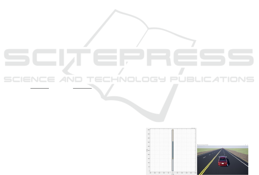
4.1.1 Straight Road

In the straight scenario, we made a velocity profile.

As it has shown in Figure 2, there were two vehicles

in the scenario that the front vehicle (the truck) had

60 km/h speed and our vehicle model was 200 meters

back of this vehicle with 80 km/h.

Figure 2: Our scenario in the drivingScenarioDesigner

schematic in MATLAB.

4.1.2 Turn

We designed the other scenario for a comparison

between our method and the other works. This

scenario consists of different turns as shown in Figure

3. The speed limit of this scenario is between 0 to 40

A Full-Featured, Enhanced Cost Function to Mitigate Motion Sickness in Semi- and Fully-autonomous Vehicles

501

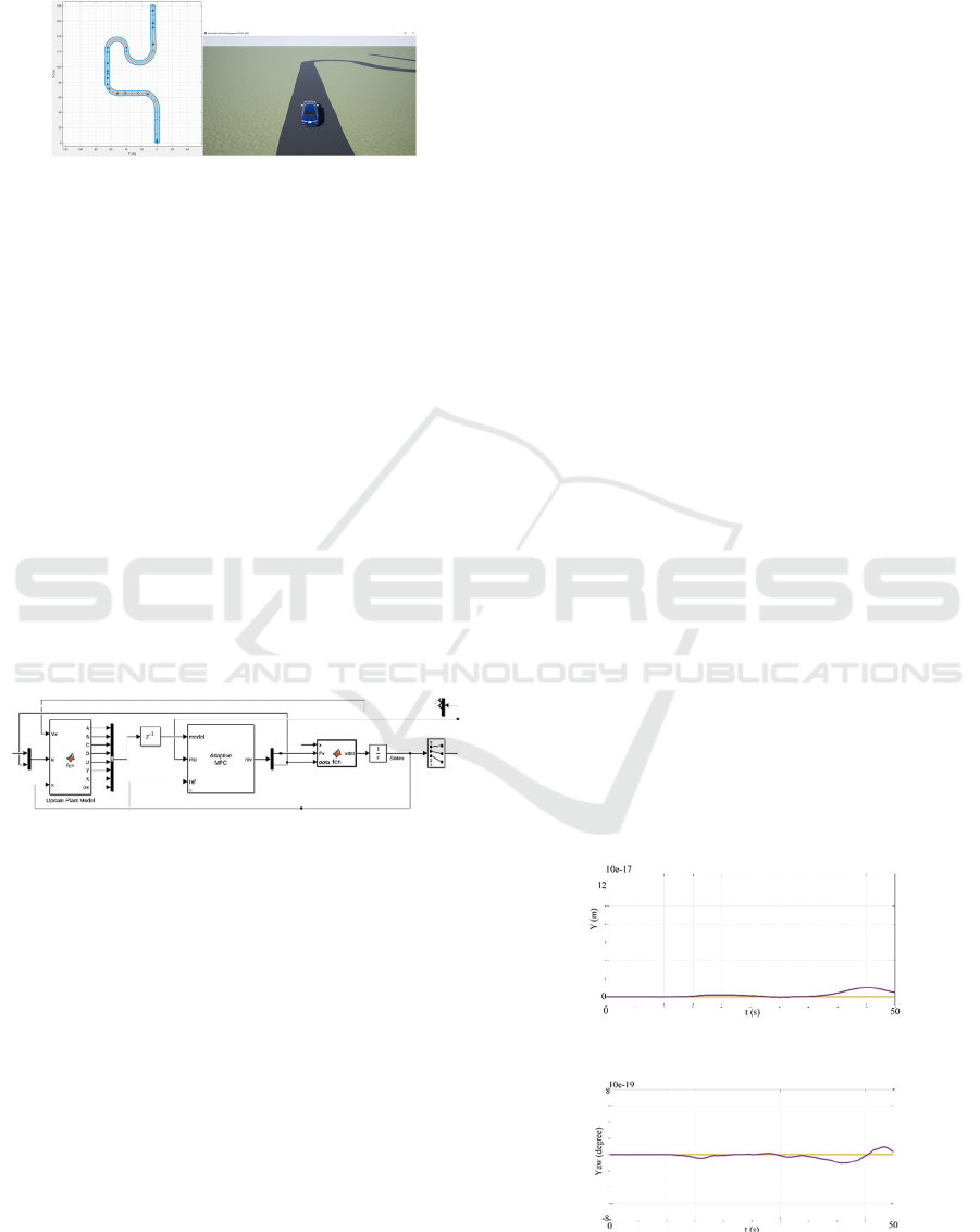
km/h and at the first, the vehicle reaches the 40 km/h

with our acceleration limitation that we discussed in

constraints.

Figure 3: The Scenario visualization in Unreal Engine.

4.2 Adaptive Model Predictive

Controller Design

We designed our AMPC using mpcDesigner

(MATLAB, 2020) and Simulink. For each time step,

our controller updated to make new states for the next

prediction horizon. In Simulink, as shown in Figure

4, we used the Adaptive MPC block for this

implementation which in it, the constraints and the

MPC parameters are attached to it by mpcDesigner

tool. The different blocks are to build the

requirements of the Adaptive MPC block. We also

brought our reference scenarios as discussed before.

The prediction horizon considered as 10 seconds and

the control horizon was 5 seconds with the sample

time of 0.1 seconds. The tuning of weights was done

by mpcDesigner tuning tool for closed-Loop

Performance and State Estimation along with

Figure 4: The Simulink implementation of Adaptive MPC.

considering the system stability. The constraints, as

discussed before, were defined in our controller using

the mpcDesigner tuning tool.

4.3 Simulator

The system is tested with the Unreal Engine simulator

(Epic Games, 2019) which connects to the Simulink.

Our simulator considered the scenario data made by

drivingScenarioDesigner, and added the output of the

system to visualize and evaluate our system.

4.4 Embedded Platform

The target embedded platform, NVIDIA Jetson AGX

Xavier is representative of the next-generation AV

Domain Controller. This platform with a GPGPU of

512-core Volta with Tensor Core and a CPU of ARM

8-core v8.2 64-bit is an appropriate choice for the AD

systems.

To have a realistic implementation, we can’t rely

on the Matlab/Simulink implementatn, and we

utilized embedded coder of MATLAB/Simulink to

convert our algorithm into C++ source code, which is

then compiled for the target platform.

5 RESULTS AND DISCUSSION

Firstly, we calculated our results regarding of the first

scenario, Straight scenario. Then, we investigated the

results of the second scenario which is Turn. Finally,

we tried to understand our timing results in the

embedded platform to be able to use it along with

other infrastructures.

We evaluated the scenarios by MSDV and IR then

we compared our work with the latest works in this

area. Our results shown different advantages

compared to the previous approaches.

5.1 Results of the Scenarios

5.1.1 Straight Road

The straight scenario included two vehicles and a

velocity profile. Our vehicle was behind a truck that

was slightly far. It started from 0 and reached 80 km/h

(22.22 m/s) and as soon as founded the distance of 5

seconds, it started slowing down to maintain the 5

seconds of the distance. Afterwards, it followed the

truck by the truck’s velocity. As shown in Figure 5,

Figure 6, and Figure 7, the output of our controller

follows the base-line with a small error.

Figure 5: The scenario (blue) and our (orange) Y.

Figure 6: The scenario (blue) and our (orange) Yaw angle.

VEHITS 2021 - 7th International Conference on Vehicle Technology and Intelligent Transport Systems

502

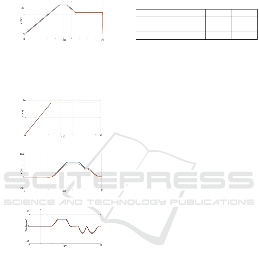
Figure 7: The scenario (orange) and our (blue) Velocity.

5.1.2 Turn

In the turn scenario, we maintained the acceleration

limitation based on AMPC algorithm designed by

Simulink and mpcDesigner. Figure 8, Figure 9, and

Figure 10 show the results.

Figure 8: The scenario (orange) and our (blue) Velocity.

Figure 9: The scenario (blue) and our (orange) Y.

Figure 10: The scenario (blue) and our (orange) Yaw angle.

5.2 MSDV and IR Analysis

Our evaluation is based on MSDV and IR. IR

generally increases overtime during a motion

sickening stimulus (Reason & Graybiel, 1969). In

(Standard, 1987), IR is considered as 0 when the

passenger feels fine, 1 with a feeling of slightly

unwell, 2 as quite ill, and 3 when the passenger is

absolutely dreadful. As shown in Table 1, the output

of the system more than having a small amount of IR

which almost is zero, it has a comparison between the

minimum IR of the previous work.

Table 1: The results of the IR evaluation.

Scenario

Time

(s)

IR (min)

Straight 50 0.07

Turn 32 0.0017

Turn in (Htike et al., 2020) 29.73 0.044

Table 1 shows that the IR of the Turn scenario is

much lower than the straight one. It is exactly what

we expected considering the accelerations used in

both scenarios since the Turn scenario has a much

lower time of accelerating.

The results show that our performance is better

since we try to use the acceleration as small as we can

and we try to make it limited to 1 m/s2. Furthermore,

our planner can make an IR near to zero. Therefore, it

has a fine feeling according to (Standard, 1987).

5.3 Embedded Platform Performance

When running on the production-like embedded

domain controller, our controller achieves 8.7 FPS,

making it suitable to interact with the other AV

components.

6 CONCLUSIONS

In this paper, we showed that by having a complex

cost function with an emphasis on Motion Sickness

Mitigation and consideration of comfort, we can

achieve a smooth controller that does not make

people sick. This work showed that the AV can have

an algorithm for Motion Sickness mitigation along

with the other tasks and make the AV more reliable

than before.

For the next works, we can add other necessary

features of AV such as LiDAR to detect and import

the data for the Motion Sickness Mitigation

Algorithm. It can finally be an algorithm which is

used with the other infrastructures.

We also plan to adopt more complex vehicle models,

such as the kinematic and dynamic model, to validate

our approach at highest speeds (i.e., > 150km/h), and

to possibly include other classes of vehicles, such as

busses and coaches, which potentially issue Motion

Sickness much more than cars.

ACKNOWLEDGEMENTS

This work was supported by the Prystine Project,

funded by Electronic Components and Systems for

European Leadership Joint Undertaking (ECSEL JU)

A Full-Featured, Enhanced Cost Function to Mitigate Motion Sickness in Semi- and Fully-autonomous Vehicles

503

in collaboration with the European Union’s H2020

Framework Programme and National Authorities,

under grant agreement n° 783190.

REFERENCES

Anon, B. (1997). Mechanical vibration and shock-

evaluation of human exposure to whole-body vibration.

Intl. Organization for Standardization, ISO, 2631.

Antonelli, D., Nesi, L., Pepe, G., & Carcaterra, A. (2019,

June). A novel approach in Optimal trajectory

identification for Autonomous driving in racetrack.

In 2019 18

European Control Conf. (ECC) (pp. 3267-

3272). IEEE.

Aswani, A., Gonzalez, H., Sastry, S. S., & Tomlin, C.

(2013). Provably safe and robust learning-based model

predictive control. Automatica, 49(5), 1216-1226.

Bellem, H., Thiel, B., Schrauf, M., & Krems, J. F. (2018).

Comfort in automated driving: An analysis of

preferences for different automated driving styles and

their dependence on personality traits. Transportation

research part F: traffic psychology and behaviour, 55,

90-100.

Diels, C. (2014). Will autonomous vehicles make us

sick? Contemporary ergonomics and human factors.

Taylor & Francis, 301-307.

Donohew, B. E., & Griffin, M. J. (2004). Motion sickness:

effect of the frequency of lateral oscillation. Aviation,

Space, and Environmental Medicine, 75(8), 649-656.

Easa, S. M., & Diachuk, M. (2020). Optimal Speed Plan for

the Overtaking of Autonomous Vehicles on Two-Lane

Highways. Infrastructures, 5(5), 44.

Elsner, J. (2018). Optimizing Passenger Comfort in Cost

Functions for Trajectory Planning. arXiv preprint

arXiv:1811.06895.

Epic Games. (2019). Unreal Engine. Retrieved from

https://www.unrealengine.com.

Filip, J. (2018). Trajectory Tracking for Autonomous

Vehicles.

Geng, K., & Liu, S. (2020). Robust Path Tracking Control

for Autonomous Vehicle Based on a Novel Fault

Tolerant Adaptive Model Predictive Control

Algorithm. Applied Sciences, 10(18), 6249.

Hajizadeh, I., Hobbs, N., Sevil, M., Rashid, M., Askari, M.

R., Brandt, R., & Cinar, A. (2020, May). Performance

Monitoring, Assessment and Modification of an

Adaptive MPC: Automated Insulin Delivery in

Diabetes. In 2020 European Control Conference

(ECC) (pp. 283-288). IEEE.

Htike, Z., Papaioannou, G., Velenis, E., & Longo, S. (2020,

May). Motion Planning of Self-driving Vehicles for

Motion Sickness Minimisation. In 2020 European

Control Conference (ECC) (pp. 1719-1724). IEEE.

Iskander, J., Attia, M., Saleh, K., Nahavandi, D., Abobakr,

A., Mohamed, S., . & Hossny, M. (2019). From car

sickness to autonomous car sickness: A review.

Transportation research part F: traffic psychology and

behaviour, 62, 716-726.

Kang, C. M., Lee, S. H., & Chung, C. C. (2014, October).

Lane estimation using a vehicle kinematic lateral

motion model under clothoidal road constraints. In 17th

International IEEE Conference on Intelligent

Transportation Systems (ITSC) (pp. 1066-1071). IEEE.

Lambert, E., Romano, R., & Watling, D. (2019, May).

Optimal path planning with clothoid curves for

passenger comfort. In Proceedings of the 5th Intl. Conf.

on Vehicle Technology and Intelligent Transport Systems

(VEHITS 2019),Vol.1, pp.609-615. SciTePress.

Luan, Z., Zhang, J., Zhao, W., & Wang, C. (2020).

Trajectory Tracking Control of Autonomous Vehicle

with Random Network Delay. IEEE Transactions on

Vehicular Technology.

MATLAB. (2020). version (R2020a). Natick,

Massachusetts: The MathWorks Inc.

Mechanical Simulation Corporation. (2020). Introduction

to CarSim.

Muske, K. R., & Rawlings, J. B. (1993). Model predictive

control with linear models. AIChE Journal, 39(2), 262-

287.

Önkol, M., & Kasnakoğlu, C. (2018). Adaptive model

predictive control of a two-wheeled robot manipulator

with varying mass. Measurement and Control, 51(1-2),

38-56.

Rajamani, R. (2011). Vehicle dynamics and control.

Springer Science & Business Media.

Reason, J. T., & Graybiel, A. (1969). Changes in subjective

estimates of well-being during the onset and remission

of motion sickness symptomatology in the slow rotation

room (Vol. 1083). US Naval Aerospace Medical

Institute, Naval Aerospace Medical Center.

Road Safety Authority, (2011). The two-second rule,

Government of Ireland.

Sivak, M., & Schoettle, B. (2015). Motion sickness in self-

driving vehicles. University of Michigan, Ann Arbor,

Transportation Research Institute.

Shi, J., Sun, D., Qin, D., Hu, M., Kan, Y., Ma, K., & Chen,

R. (2020). Planning the trajectory of an autonomous

wheel loader and tracking its trajectory via adaptive

model predictive control. Robotics and Autonomous

Systems, 103570.

Standard, B. S. I. (1987). 6841, Guide to Measurement and

Evaluation of Human Exposure to Whole-Body

Mechanical Vibration and Repeated Shock. London,

UK: BSI.

Wu, J., Wang, Z., & Zhang, L. (2020). Unbiased-

estimation-based and computation-efficient adaptive

MPC for four-wheel-independently-actuated electric

vehicles. Mechanism and Machine Theory, 154,

104100.

Yimer, T. H., Wen, C., Yu, X., & Jiang, C. (2020). A Study

of the Minimum Safe Distance between Human Driven

and Driverless Cars Using Safe Distance Model. arXiv

preprint arXiv:2006.07022.

VEHITS 2021 - 7th International Conference on Vehicle Technology and Intelligent Transport Systems

504