
Study of Stability through Lyapunov Theory and Passivity following
a FDI on a Velocity Control System
*
M. Ruhnke
1,2
, X. Moreau
2
, A. Benine Neto
2
, M. Moze
1
, F. Aioun
1
and F. Guillemard
1
1
Stellantis, Centre Technique de Vélizy, Route de Gisy, 78140 Vélizy-Villacoublay, France
2
Univ. Bordeaux, CNRS, Bx INP, Laboratoire IMS, UMR 5218, 33400 Talence, France
Keywords: Passivity, Switched Systems, Dissipativity, Vehicle Dynamics, Reconfiguration.
Abstract: Ensuring safety and fault tolerant strategies is essential in the development of Advanced Driver Assistance
System, such as an automated cruise control.This work presents a study of the stability of switched regulated
systems following the reconfiguration of the speed controller due to a fault.
Firstly, the context of these works is presented highlighting the need to have a fault management system with
a diagnostic part and a reconfiguration part in order to ensure the operating safety. The reconfiguration part
can take the form of a switch thus involving the study of stability. It is in this context that, secondly, the
passivity of the plant as well as of both the controllers (CRONE and PI) is demonstrated.
As the switch takes place between two elements of a passive nature, the last point of this work highlights the
application of the continuous approach in order to demonstrate the passivity and therefore the stability of the
regulated plant despite the presence of the switch.
To address this problem, an augmented model in the form of a generic state space representation of the
controllers and the plant is constructed. Then, a Lyapunov candidate function representing the sum of the
storage function of the controller and the plant is defined. A sign study of this function as well as its derivative
is carried out for the two operational modes (CRONE regulating the plant and PI regulating the plant) in order
to demonstrate the passivity of the switched regulated systems.
1 INTRODUCTION
Nowadays, research and development of Advanced
Driver Assistance Systems (ADAS) in the automotive
field focus on the development and integration of
increasingly complex autonomous functions.
However, one of the main factors to take into
account in the development of these functions is to
ensure the safety of the passengers at all times. For
this, the good functioning of the various systems
present within the Automated Driving (AD) must be
ensured.
Tools have therefore been put in place to prevent
the presence of any faults or failures that could have
disastrous consequences for the system and endanger
the passengers of the vehicle. These tools are mainly
Fault Detection and Isolation (FDI) methods. These
are part of the fault management procedures.
*
This work is supported by Stellantis OpenLab program
(Electronics and Systems for Automotive).
FDI methods are classified in two categories:
qualitative methods and quantitative methods (Jones
et al, 1988). The first one is based on data history. The
most known methods are using artificial intelligence
or fuzzy logic (Franck et al, 1997), neural network or
genetic algorithms (Samanta, 2004) and so on. The
second category is based on mathematical model of
the system. The main methods are the parity spaces
ones (Evans et al, 1970; Potter et al, 1977; Daly et al,
1979), the parametrical estimations ones (Isermann,
1984; Isermann, 2006; Constantinescu et al, 1995)
and the state estimations ones (Beard, 1971;
Massoumnia, 1986; Edelmayer et al, 1996).
Application on the automotive field focus mainly
on mechanical faults such as internal combustion
engine (Kim et al, 1998), drive-by-wire (Isermann &
al, 2002) or detection of non-aligned wheels or
degraded braking (Spooner et al, 1997).
After the fault detection, the important point for
122
Ruhnke, M., Moreau, X., Neto, A., Moze, M., Aioun, F. and Guillemard, F.
Study of Stability through Lyapunov Theory and Passivity following a FDI on a Velocity Control System.
DOI: 10.5220/0010444801220132
In Proceedings of the 7th International Conference on Vehicle Technology and Intelligent Transport Systems (VEHITS 2021), pages 122-132
ISBN: 978-989-758-513-5
Copyright
c
2021 by SCITEPRESS – Science and Technology Publications, Lda. All rights reserved

the safety and the good functioning is to ensure, that
despite the presence of the fault, the system continues
to operate, either in an operational way or in a
degraded way. For this, a reconfiguration is required
in order to switch from the defective component or
function to the operational or degraded one. It is from
this perspective of reconfiguration that switched
systems are interesting to set up.
However, from a control engineering perspective
and above all regarding stability, switching can cause
instabilities within the system and therefore present
risks.
To ensure the stability requirements, tools based
on Lyapunov’s stability have been put in place.
Before presenting a state of the art of the existing
methods to guarantee the stability of switched
systems, Lyapunov’s theory is first recalled. Indeed,
the majority of stabilization methods are based on the
Lyapunov criterion.
1.1 Lyapunov Stability Criterion
By definition, a stable system is a system which,
when removed from its position of equilibrium tends
to return to it.
One of the major theories in the study of the
stability of systems is Lyapunov’s theory of stability.
The main advantage of this theory is that it has an
application to both linear and nonlinear systems.
The Lyapunov stability criterion is based on a
candidate state function denoted representing
the energy of the system studied. The latter must be
defined positive and its derivative, which is
representing the evolution of the energy over time,
must be defined negative. This means that the energy
of the system is positive but decreases with time. As
a result, the system returns to a rest position, so it is
stable. These conditions can be written in the form of
inequalities as defined below:
(1)
and
, (2)
where, represents the state vector.
1.2 State of Art of Stability Methods
for Switched Systems Methods
Consider a state vector
, an input vector
and an output vector
with
being a time index.
Let
with , the number of
subsystems. is a piecewise constant function whose
value changes at the switching times. This function is
called the commutation law.
A switched discrete time system can be described
by the following equations:
(3)
In the literature, methods for studying the stability
of switched systems, in particular for discrete time
systems, have been implemented. The definition of
the joint spectral radius presented in (Hetel et al,
2007, Tsitsiklis et al, 1997) is one of these methods
and gives a sufficient and necessary condition for the
stability of the system by computing the extension of
the radius of a set of matrices
,
denoted . The major difficulty of this method is
to compute numerically the joint spectral radius in a
generic framework. Several approximations are made
in the literature.
Other methods are based directly on the Lyapunov
candidate function . In (Shorten & al, 2007;
King et al, 2004; Zhai & al, 2002), the principle of a
common quadratic Lyapunov function (CQLF) is
proposed for continuous second or even third order
systems and also give algebraic criteria in order to
determine this function. The principle is based on the
existence of a Lyapunov function of a quadratic form
and common to each subsystem.
However, it is in general very difficult to obtain
such a function and its use is restricted to relatively
low order systems.
In order to overcome the constraints of a
Lyapunov function common to each subsystem,
works presented by (Mignone et al, 2000; Daafouz et
al, 2002) highlight the use of a multiple Lyapunov
functions. In the case of discrete time systems, a poly-
quadratic Lyapunov function is presented. In this
method, each subsystem has a Lyapunov function
, which satisfies linear matrix inequalities in
order to prove the existence of a poly-quadratic
Lyapunov function and therefore the stability of the
switched system.
Whatever the methods presented above, they are
based on matrix algebra specific to the systems
studied. This therefore assumes knowledge of the
system model.
However
, in cases that are more
complex, obtaining the mathematical model of the
plant is very difficult or even impossible, particularly
in cases such as a switch between “black box” type
systems or AI algorithms.
Study of Stability through Lyapunov Theory and Passivity following a FDI on a Velocity Control System
123

Hence, the definition of a generic stability
criterion for switched systems, which is not necessary
based on the knowledge of the mathematical model,
is required. It is with this in mind that the notion of
passivity and its implication with stability are defined
and used for the work presented in this paper. In the
next subsection, the notion of passivity is thus
presented.
1.3 Notion of Passive Systems
Passivity makes it possible to characterize a system
based on the notion of energy (McCourt et al, 2010).
Definition 1: Let define a causal continuous-time
system denoted , with input vector
and
output vector
. This system is said to be
passive if , the variation of its stored energy
over time noted
is less than the power supplied
by its input, i.e.:
. (4)
Remark 1.1: The input vector included all the
inputs of the system, i.e. the control inputs and the
disturbances.
Remark 1.2: Each output is associated with its
respective input as part of the power calculation.
Otherwise, passivity cannot be guaranteed.
Remark 1.3: For an energy point of view, passivity
implies that the energy stored by a system denoted
dissipates and therefore decreases over time.
Thus, the Lyapunov stability criteria are verified.
According to (Khalil, 2002), a passive system is
therefore a stable system in the sense of Lyapunov but
the converse is not true.
Remark 1.4: In addition, the advantage of using
passivity is that the interconnection of passive
systems (in parallel and in feedback) is passive. The
proofs are demonstrated in (McCourt et al, 2012).
This characteristic is very interesting specially in the
case of hybrid systems.
The state of the art on the methods on the stability
of switched systems are mainly based on the
knowledge of a mathematical model, which can be
difficult or even impossible to obtain, hence the need
to focus on another approach. Passivity and its link
with stability as well as its application for
interconnected systems offer a good alternative for
the stability of switched systems.
The work is therefore presented as follows.
Section 2 recalls the study framework, in particular
the detection of the fault on one of the controller in
the velocity control, which is at the origin of the
switch. The passivity of the plant, modelled by a
longitudinal bicycle model is then studied as well as
the passivity of both of the controllers: CRONE and
PI. The different proofs of passivity lead to the
conclusion that the switched system switches
between two passive subsystems. Section 3 then,
introduce the principle of continuous approach and
allows to conclude of the stability of the switch.
2 STUDY OF PASSIVITY
This section mainly focuses on the analysis of the
passivity of the plant, modelled by a longitudinal
bicycle model, as well as of the two controllers
present within the speed controller.
First, the study framework is recalled in order to
determine the origin of the switch. Then, an analysis
of the passivity of the plant through the analysis of the
analytical expressions of the nonlinear model is
made. The linear case is presented in order to
introduce the different expressions necessary for the
study of stability in Section 3.
Finally, this section presents the analysis of
passivity for a 2
nd
generation CRONE controller and
a PI controller.
2.1 Study Framework
The work presented in this paper follows the
development of a fault-tolerant strategy for an
automotive cruise control detailed in (Ruhnke & al,
2020).
As a reminder, this work consists of regulating the
longitudinal speed around a reference value using the
CRONE controller. This latter undergoes at an
arbitrary time
a sampling fault, which forces its
output value to an erroneous value. This has the
consequence to fault the speed regulation.
The objective is therefore to design a supervisor,
which makes it possible both to detect the fault on the
CRONE controller and, following the detection, to
switch to a functional PI controller in order to ensure
the good functioning of the velocity control system.
The block diagram of the system is illustrated Figure
1.
VEHITS 2021 - 7th International Conference on Vehicle Technology and Intelligent Transport Systems
124
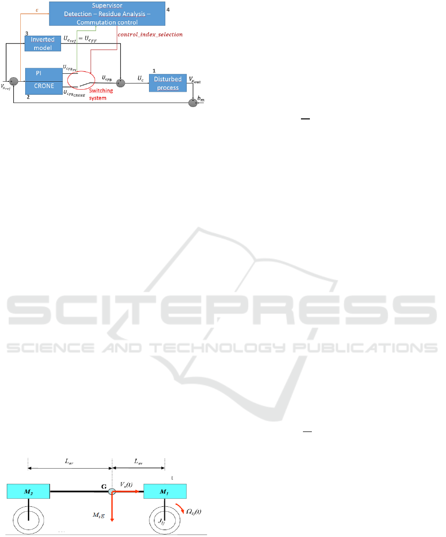
Figure 1: Block diagram of the studied system.
2.2 Plant Analysis
In order to analyse the passivity of the plant, the
nonlinear model is first presented as well as the
simplifying hypotheses linked to the study
framework. The analytical expression of the variation
of the storage function is then defined followed by
sign study.
2.2.1 Context
For this work, it is assumed that the longitudinal
speed is regulated around a reference speed
.
The vehicle is an urban electrical vehicle with two
in-wheel motors in the front wheel. This vehicle is
supposed to drive in a straight line on a horizontal dry
road. The total mass of the vehicle
is evenly
distributed throughout the vehicle.
In this paper, a simplified driving scenario is
studied. Thus, the plant does not undergo disturbance.
In the following notations, index indicates
whether if it is the front wheels or the rear
wheels , which are considered, and the index
indicates whether if it is the left wheels or the
right wheels , which are considered.
For the modelling of the vehicle, the longitudinal
bicycle model is used and is illustrated Figure 2.
Figure 2: Longitudinal model of the vehicle.
and
represents respectively the rear and the
front wheelbase.
and
are respectively the front
and rear masses. is the center of gravity of the
vehicle and the gravitational force.
and
are defined below in the expression of the
equations of the model.
Following the various simplifying assumptions,
only the longitudinal dynamics are considered. By
applying the fundamental principle of dynamics, the
plant can be modelled through the expressions of the
longitudinal velocity
and the wheel rotation
speeds
. The two quantities are expressed in the
absolute reference, such as:
(5)
where,
represents the total mass of the vehicle and
is the sum of the longitudinal forces, which is
expressed in its general form as follows:
. (6)
are the longitudinal nonlinear forces
expressed by the Pacejka model (Morand & al, 2015)
for one wheel. The forces developed by the left front
tire
are equal to the forces developed by the
right front tire
, so the following notation is
applied:
.
and
are the aerodynamic and the
rolling resistance forces and
represents the
force associated with the gust of wind.
As the disturbance
is not considered for
the analysis of passivity in the nonlinear case,
expression (6) can be rewritten as follows:
. (7)
Regarding the wheel rotation dynamics, only the
two front driving wheels are considered. The rotation
speed of the wheels can therefore be written as
follows:
. (8)
is the moment of inertia and
is the sum
of the momentum applied on the front wheels. The
sum is expressed as follows:
, (9)
where,
represents the motor torque and the
control command,
, the viscous friction and
, the resistant momentum. For more
information, (Morand & al, 2015) provides a more
detailed model.
Rear
Front
Road
Study of Stability through Lyapunov Theory and Passivity following a FDI on a Velocity Control System
125

2.2.2 Nonlinear Case without Disturbance
For simplifying the notation, temporal index will not
be written in the following expressions and
is
rewritten as .
In order to analyse the passivity of the plant, the
storage function must be defined. In this case, it
is equal to the sum of the kinetic energies of the
system and the potential energy of gravity, which is
here constant and denoted , that is:
. (10)
By deriving equation (10),
is equal to:
, (11)
where,
(12)
and
. (13)
and
are replaced in (11) by their respective
expressions:
. (14)
By expanding equation (14),
can be expressed
as follows:
, (15)
where,
represents the input/output product
associated with the power calculation,
is the
power lost to rotation and
is the
power lost to translation.
According to equation (4), the plant is considered
as passive if the following inequality holds:
. (16)
As the vehicle moves forward and the variables
are expressed in the absolute coordinate system, the
sign of these latter is known.
Thus, for the driving scenario under study,
and
are positive as well as the
module of
and
. Since
and
are
positive, this implies that
are thus positive.
Therefore, validation of inequality (16) depends
on the sign of:
, (17)
which can be rewritten as:
. (18)
In order to define the sign of (18), the expression
of the slip rate in traction,
, is recalled.
. (19)
As the vehicle moves forward,
is positive.
By isolating the numerator of (19), the following
equation is as follows:
. (20)
As a result,
is negative as well as
equation (18).
Inequality (16) is therefore respected and the plant
is passive.
2.2.3 Linearized Model of the Plant
In this subsection, the expression of the linearized
model of the plant as well as the expression of the
storage function and its derivative are presented.
The objective is not to demonstrate the passivity
of the plant in the linear case, but to introduce the
matrices of the linearized model and the expression
of the storage function of the plant, which are
necessary for the approach developed in Section 3 for
the proof of the stability of the switched system.
For this purpose, a linearization of equations (12)
and (13) around an operational point is made.
A linear state space representation is obtained by
linearization of equations (12) and (13) around an
equilibrium point denoted
, where
represents the reference longitudinal speed and
, the wheel rotation speed of reference associated
with
. Thus, the matrices A, B, C and D of the
state space representation are as follows (Morand &
al, 2015):
, (21)
and
,
(22)
with
,
and , representing
respectively the small variations around the
equilibrium point for the state, the input and the
output vectors of the linearized model.
The expression of the storage energy can be
rewritten in the linear case, such as:
VEHITS 2021 - 7th International Conference on Vehicle Technology and Intelligent Transport Systems
126

. (23)
By deriving expression (23) and replacing the
expressions of
and , the derivative of the storage
function is equal to:
. (24)
By expanding the expression (24),
, (25)
where
represents the input/output product.
To simplify the notations, equation (25) is
rewritten as follow:
, (26)
with,
and
.
The next step is to verify the passive nature of the
CRONE controller and the PI controller. This
analysis will lead to the conclusion that the switch
takes place between two passive subsystems.
2.3 Passivity of the Controllers
In order to study the passivity of CRONE and PI
controllers, Definition 1 is applied.
For both controllers, the expression of the transfer
function as well as the Partial Fraction
Decomposition (PFD) are defined. A causal diagram
of the PI controller and of one of the cell of the
CRONE controller are illustrated. Finally, the
passivity of each controller is studied.
As a reminder, a system is passive if the following
inequality is respected:
. (27)
where
represents the input/output product
associated with the power calculation.
2.3.1 Passivity of the PI Controller
The transfer function of the PI controller is of the
following form:
. (28)
The PFD of transfer function (28) can be written as
follows:
, (29)
with
.
The input of the controller is the error signal
and the output is
associated with a voltage and
proportional to the motor torque
through a
factor .
The causal diagram associated with the parallel
form of the PI is illustrated Figure 3.
Figure 3: Causal diagram associated with the parallel form
of the PI controller.
In order to study the controller’s passivity, the
storage function must be defined. In the case of the
PI, the energy is stored only in the integral element,
so is expressed as follows:
. (30)
The next step is to derive equation (30) to check
if inequality (27) is respected.
Thus,
, (31)
where,
(32)
and
. (33)
By replacing
and
in (33),
can be
rewritten as,
. (34)
As
, by developing and
rewriting (34),
is equal to:
, (35)
where,
represents the
input/output product associated with the power
calculus;
The PI is passive if the following inequality holds:
. (36)
As
is always
Study of Stability through Lyapunov Theory and Passivity following a FDI on a Velocity Control System
127
positive, inequality (36) is always respected and
therefore the PI controller is passive.
2.3.2 Passivity of the CRONE Controller
The CRONE controller is a 2
nd
generation CRONE. It
was calculated from the loop-shaping of the open
loop. For more information about the design of the
CRONE controller (Morand et al, 2015) presents the
different stages of the design.
The rational form of the controller has two parts:
an integer part and a part, which represents the
rationalization of the phase lead cell of non integer
order rewritten as a recursive product of zeros and
poles. The expression of the transfer function of the
rational form of the controller is the following:
. (37)
The PFD of the transfer function (37) is expressed
as follows:
, (38)
with
.
By posing
, with
, the expression
(41) can be rewritten such as,
. (39)
The input of the controller is the error signal and
the output is
associated with a voltage and
proportional to the motor torque
through a
factor .
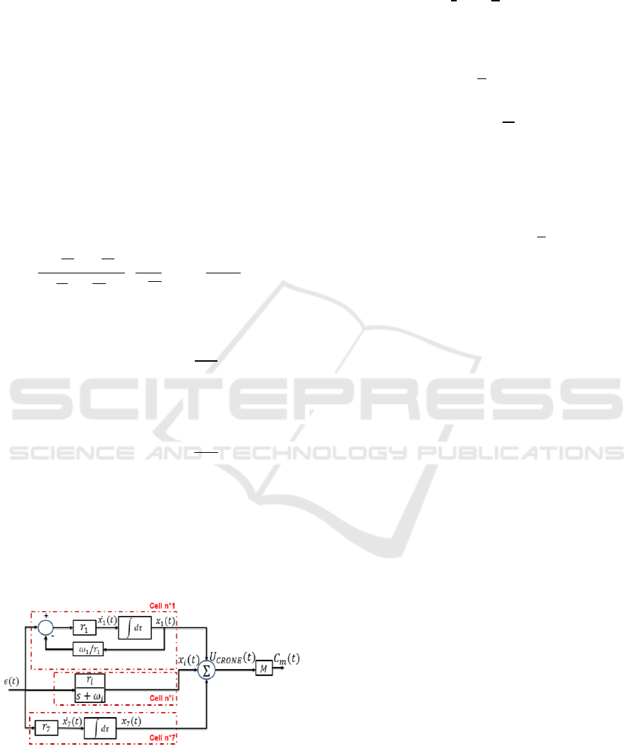
The causal diagram associated with the parallel
form of the rational form of the CRONE is
illustrated Figure 4.
Figure 4: Causal diagram of the parallel form of the rational
form of the CRONE controller.
For the study of the passivity of the controller, the
storage function is defined. As the energy is only
stored in the integral elements,
is defined as
follows:
. (40)
The derivative of the storage function is then
equal to:
, (41)
where,
. (42)
By replacing
by its expression,
, (43)
where,
,
(44)
which represents the input/output product associated
with the power calculus.
For the CRONE to be passive, the following
inequality must hold:
. (45)
However,
(46)
and
thus inequality (45) holds and the
CRONE controller is passive.
During Section 2, the passivity plant was shown
as well as the passivity of both of the controllers
through the analysis of analytical expressions.
The problem is the following: the fault detection
has caused a switch, which takes place between two
passive subsystems. It is, thus, necessary to prove the
stable nature of the switching system in order to
ensure the system’s operating safety.
3 STABILITY OF THE
SWITCHED SYSTEMS
The previous sections made it possible to demonstrate
that the switch was done between two passive
subsystems, namely on the one hand, the longitudinal
model regulated by the CRONE and on the other
hand, the longitudinal model regulated by the PI.
The objective is to prove the overall stability of
the longitudinal speed controller, whatever the
switching law.
VEHITS 2021 - 7th International Conference on Vehicle Technology and Intelligent Transport Systems
128

For this, the continuous approach method
(Nouillant et al., 2001) is developed. The principle is
to build a state space representation of an augmented
model, here the linearized model of the plant and the
regulation, regardless the operating mode. In
addition, only one Lyapunov candidate function
denoted is constructed.
The objective is to verify that the Lyapunov
candidate function satisfies, for each operating mode,
the Lyapunov criteria represented by equations (1)
and (2) namely
and
.
If this is the case, the candidate function is a
Lyapunov function common to both subsystems and
the following theorem can be applied:
Theorem 1: (Boyd & al, 1994) (Sun and Ge, 2011).
Let be the linear switched system
. If
there exists a positive definite symmetric matrix
such that the following inequality is respected:
, (47)
then the function
is a Common
Quadratic Lyapunov Function (CQLF) for the
system. The switching system is then stable whatever
the switching law.
Remark 3.1: This theorem is a sufficient condition but
very conservative because it is difficult to obtain such
a function.
The matrices
and
of the augmented model
are defined. In order to have a generic writing the
matrices are defined in the most complex case, i.e. by
taking into account the largest state and command
vectors.
For this, the following state vector is
considered:
where
represent the states of the regulation
and
respectively the longitudinal speed and the
wheel’s rotation speed, represent the states of the
plant in the linearized model. In addition, the input
vector is considered
, which represent the
reference longitudinal speed.
The matrices
and
are as follows:
, (48)
where, and represents the matrix of the
linearized model of the plant (see equation (21)).
. (49)
Index represents the operating mode in which the
system is, i.e.:
• If , the CRONE is in operation and
regulates the system, thus
and
have the numerical values associated with
the PFD of the CRONE controller and .
• If , the PI is in operation and regulates
the systems, thus
,
,
and
.
In order to study the stability of the switched system,
the energy storage function is defined and denoted
. This function is equal to the sum of the energy
storage function of the regulation system and the
energy storage function of the plant.
. (50)
This function can be rewritten under a matricial form
such as:
, (51)
where,
with
.
is considered as the candidate Lyapunov
function.
The objective is to calculate the derivative of
and to check if it meets the Lyapunov criteria
for both operating mode.
,
(52)
where,
for
and
.
By replacing
,
and with their respective
expressions, equation (52) can be rewritten as :
. (53)
Study of Stability through Lyapunov Theory and Passivity following a FDI on a Velocity Control System
129

Equation (53) can be decomposed in two
functions:
, which represents the derivative
of the storage function for the regulation
and
, which represents the derivative of the
storage function for the plant.
. (54)
, (55)
In order to check if the candidate function
is
a Lyapunov function, the sign of (50) is first studied
for both case.
When , the CRONE is regulating the system.
Moreover,
and according to
section 2.3,
.
As a result, is positive definite.
When , the PI is regulating the system. Thus,
equation (50) can be rewritten such as:
. (56)
As
,
is positive definite.
At this stage, in order to conclude on the nature of
the candidate function , the sign of (53) has to be
studied. For this purpose, the sign of (54) and (55) are
studied for both functioning cases.
For the first case, when ,
. As
, the function
is negative definite.
For the second case, when ,
,
then
is negative definite.
Despite the operating mode, the derivative of the
storage function for the controller is always defined
negative. Therefore the sign of (53) depends on the
sign of (55), which is independent of the functioning
mode.
Lemma 3.1: (Khalil, 2002). If a system is passive
with a positive storage function , then the origin
is stable is the sense of Lyapunov by considering
as a Lyapunov function candidate.
Then,
.
The approach presented in section 2.2.2 and 2.2.3
shows that firstly the plant is passive and secondly
that both
and
are positive. As a result,
the storage function of the plant, which is
is positive definite. By
using Lemma 3.1, equation (55) is then negative
definite.
Equations (54) and (55), which respectively
represents the derivative of the storage function for
the controller and the plant are both negative definite.
In this case, equation (53), which represents the sum
of these two functions is as well negative definite.
Since the candidate function is positive
definite and its derivative is negative definite for both
operating modes, is therefore a common
quadratic Lyapunov function. As the result, by
application of Theorem 1, the regulated longitudinal
model is stable.
4 CONCLUSIONS
Fault management systems are employed to ensure
the operational safety of the Advanced Driver
Assistance Systems. These include a diagnostic part
that detects and locales the fault, and a
reconfiguration part that follows the detection,
allowing you to switch to a functional mode or a
degraded mode. The reconfiguration can take the
form of a switch. As the latter can be a source of
instabilities, it is therefore necessary to ensure the
stability of the overall system despite the presence of
switching.
Thus, the purpose of this work was to study the
stability of switched regulated systems following
reconfiguration due to the detection of a fault on the
calculator of the Automated Cruise Control system.
In order to answer this problem, the passivity of
the undisturbed plant modelled by a longitudinal non-
linear bicycle model, as well as the Partial Fraction
Decomposition of the PI and CRONE controllers,
was studied in section 2.
For the plant, the passivity was demonstrated
through the sign study of the analytical expression of
the storage function as well as its derivative. The
same approach was applied to de Partial Fraction
Decomposition of both controllers.
The study of passivity concludes that the switch
occurs between two passive subsystems, namely the
plant controlled by the CRONE and the plant
controlled by the PI.
Finally, in order to show the passive and therefore
stable nature of the switched regulated systems, the
continuous approach has been developed. The latter
consists in building an augmented model through a
state space representation whose structure is
independent of the operating mode. This state space
representation contains the controllers and the plant.
Then, a single candidate function of Lyapunov is
defined and represents the sum between the storage
function of the regulation and the storage function of
the plant. A sign study of this function and its
derivative leads to the conclusion that the candidate
function meets Lyapunov’s stability criteria and
VEHITS 2021 - 7th International Conference on Vehicle Technology and Intelligent Transport Systems
130

therefore that the regulated longitudinal bicycle
model is passive and thus stable, despite the switch
between CRONE and PI controllers.
The safety and security aspect have been proven
through these works. The perspectives, however,
related to an aspect of comfort.
Indeed, when the CRONE controller is
operational, the PI operated in open loop. In some
cases, the switch can generate a significant
discontinuity in the control signal. These abrupt
variations can engender sources of discomfort for the
passengers, particularly in terms of sudden variation
of acceleration.
Regarding the application area, this work was
developed around a longitudinal model without
disturbances and on a dry, straight and plane road. It
would be interesting in terms of perspectives, to
expand the model used, to make it more realistic and
generic with regard to real driving scenarios.
On the one hand, disturbances such as gusts of
wind, slopes of the road, poor road adherence or non-
uniform loading can be considered and the other
hand, other vehicle-specific dynamics such as lateral
and yaw dynamics can be taken into account.
Then, a study of the stability associated with
reconfiguration, regardless of driving scenarios,
would allow verifying the genericity of the
reconfiguration.
In the longer term, the idea is to study
reconfiguration and stability on the architecture of the
Automated Driving that is more complex with an
application on driving-aid functions such as artificial
intelligence-based decision-making or planning
algorithms whose mathematical model is more
difficult even impossible to obtain.
These perspectives will enhance the operating
safety of the generic architecture of an Automated
Driving vehicle in both highway and urban
environments.
REFERENCES
Beard, R.V, 1971. Article. Failure accommodation in
linear systems through self-reorganization, Rapport
technique. Man. Vehicle Lab, MIT.
Boyd, S., El Ghaoui, L., Feron, E., Balakrishnan, V., 1994.
Article. Linear Matrix Inequalites in Systems and
Control Theory. SIAM Studies in Applied Mathematics.
Constantinescu, R.F., Lawrence, P.D., Hill, P.G., Brown,
T.S., 1995. Article. Model-based fault diagnosis of a
two-stroke diesel engine. IEEE International
Conference on Systems, Man and Cybernetics.
Daafouz, J., Riedlinger, P., Iung, C., 2002. Article. Stability
analysis and control synthesis for switched systems: A
switched Lyapunov function approach. IEEE
Transactions on Automatic Control, 47, pages 1883-
1887.
Daly, K.C., Gai, E., Harrison, J.V., 1979. Article.
Generalized likelihood test for FDI redundancy sensor
configurations. Journal of Guidance and Control (2)1.
Edelmayer, A., Bokor, J., Keviczky, L., 1996. Article.
detection filter design for linear systems: Comparison
of two approaches. In Proceeding of the 13
th
IFAC
World Congress, USA.
Evans, F.A., Wilcox, J.C., 1970. Article. Experimental
strapdown redundant sensor inertial navigation system.
Journal of Spacecraft 7(9).
Franck, P.M., Koppen-Seliger, B., 1997. Article. Fuzzy
logic and neural network applications to fault
diagnosis. International Journal of Approximate
Reasoning, vol.16, no.1, pages 67-88.
Hetel, L., Daafouz, J., Iung, C., 2007. Article. Equivalence
between the Lyapunov-Krasovkii functional approach
for discrete delay systems and the stability conditions
for switched systems. IFAC Proceedings Volumes,
Vol.40. Issue 23.
Isermann, R., 1984. Article. Process Fault diagnosis based
on modelling and estimation methods – A survey.
Automatica, vol.20, pages 287-404.
Isermann, R., Schwarz, R., Stolzl, S., 2002. Article. Fault-
tolerant drive-by-wire systems. IEEE Control Systems,
22(5), pages 64-81.
Isermann, R., 2006. Fault diagnosis systems: an
introduction from fault detection to fault tolerance.
Springer.
Jones, A.H., Porter, B., Fripp, R.N, 1988. Article.
Qualitative and quantitative approaches to the
diagnosis of plan faults. Proceedings IEEE
International Symposium on Intelligent Control, 24-26.
Khalil, H.K., 2002. Nonlinear Systems. Prentice Hall, 3
rd
Edition.
Kim, Y.W., Rizzoni, G., Utkin, V., 1998. Article.
Automotive engine diagnosis and control via nonlinear
estimation. IEEE Control Systems, 18(5), pages 84-99.
King, C., Shorten, R., 2004. Article. A singularity test for
the existence of common quadratic Lyapunov functions
for pairs of stable lti systems. In Proceedings of the
American Control Conference, pages 3881-3884.
Li, J., Zhao, J., Chen, C., 2016. Article. Dissipativity and
feedback passivation for switched discrete-time
nonlinear systems. System & Control Letters, Vol. 87,
pages 47-55.
McCourt, J., Antsaklis, P.J., 2010. Article. Stability of
Networked Passive Switched Systems. 49
th
IEEE.
Conference on Decision and Control.
McCourt, J., Antsaklis, P.J., 2012. Article. Stability of
Interconnected Switched Systems using QSR
Dissipativity with Multiple Supply Rates. (ACC)
American Control Conference.
Massoumnia, M.A., 1986. Article. A geometric approach to
the synthesis of failure detection filters. IEEE
Transactions on Automatic Control 31(9), pages 839-
846.
Study of Stability through Lyapunov Theory and Passivity following a FDI on a Velocity Control System
131

Mignone, D., Ferrari-Trecate, G., Morari, M., 2000. Article.
Stability and stabilization of piecewise affine and
hybrid systems: A LMI approach. Proceedings of the
39
th
Conf. on Decision and Control, pages 504-509.
Morand. A., Moreau. X., Melchior, P., Moze. M.,
Guillemard. F., 2015. Article. CRONE Cruise Control
System, IEEE Transaction on Vehicular Technology,
ISSN: 0018-9545, DOI: 10.1109/TVT.2015.2392074,
Vol. 65, N°1, pages 15-28.
Nouillant, C., Moreau, X., Oustaloup, A., 2001. Article.
Hybrid Control of a semi active suspension system. ATT
Congress & Exhibition 2001, Vol.6: Chassis and Total
Vehicle, pages 45-50.
Potter, J.E., Suman, M.C., 1977. Article. Thresholdless
redundancy managements with arrays of skewed
instruments. Integrity in electronic flight control
systems, pages. 1-25.
Ruhnke, M., Moreau, X., Benine-neto, A., Moze, M.,
Aioun, F., Guillemard, F., Rizzo, A., 2020. Article.
Fault tolerant velocity control of an urban autonomous
vehicle based on a switching strategy. 28
th
Mediterranean Conf. on Control and Automation.
Samanta, B., 2004. Article. Gear fault detection using
artificial neural networks and support vector machines
with genetic algorithms. Mechanical Systems and
Signal Processing, vol.18, no.3, pages 626-644.
Shorten, R., Wirth, F., Mason, O., Wulff, K., King, C.,
2007. Article. Stability criteria for switched and hybrid
systems. Invited paper for SIAM Review.
Spooner, J.T., Passino, K.M., 1997. Article. Fault-tolerant
control for automated highway systems. IEEE
Transaction on vehicular technology, 46(3), pages 770-
785.
Sun, Z., Ge, S.S., 2011. Book, Stability Theory of Switched
Dynamical Systems, Springer.
Tsitsiklis, J., Blondel, V., 1997. Article. The Lyapunov
exponent and joint spectral radius of pairs of matrices
are hard when not impossible to compute and to
approximate. Mathematics of Control, Signals, and
Systems, 10, pages 31-40.
Zhai, G., Hu, B., Yasuda, K., Michel, A.N., 2002. Article.
Qualitative analysis of discrete-time switched systems.
In Proceedings of the American Control Conference,
vol. 3, pages 1880-1885.
Zhao, J., Hill, D.J., 2005. Article. Dissipativity Theory for
Switched Systems. 44
th
IEEE Conference on Decision
and Control, and the European Control Conference.
VEHITS 2021 - 7th International Conference on Vehicle Technology and Intelligent Transport Systems
132
