
Traffic Congestion “Gap” Analysis in India
Tsutomu Tsuboi
a
and Tomoaki Mizutani
Nagoya Electric Works Co. Ltd., 29-1 Mentoku, Shinoda Ama-shit, Aichi, Japan
Keywords: Traffic Flow, Traffic Congestion, Developing County, Traffic Jam.
Abstract: This study is more than one-month traffic flow observation in India and introduces new traffic congestion
“Gap” from the analysis of real traffic flow analysis in India. Traffic congestion becomes serious problem
especially in developing countries such as India. In general, it is quite challenging to collect traffic data and
understand traffic congestion problem from its data analysis. In this study, it is the first time to show long
term traffic monitoring at one of major junction in Ahmedabad city of Gujarat state India. IAs for traffic
congestion analysis, the following challenges are executed with a collaboration from local city government.
Step 1 is to select location for 8 months observation by traffic monitoring camera in the city. Step 2 is to
analyse traffic flow at the junction from each direction traffic flow. Step 3 is to evaluate traffic congestion
with traffic flow parameter from traffic flow theory. Step 4 is to analyse geographical mapping by GIS tool.
Based on these steps, it reached to unique traffic congestion mechanism in the junction, which it is named
congestion “Gap” and large traffic volume is not always a case of traffic congestion. From this result, there is
a possibility to improve traffic management when more detail observation at certain time of traffic congestion
happing and environmental condition such as traffic signal control, road infrastructure structure and so on.
1 INTRODUCTION
This study is a series of the traffic flow analysis in
India under India and Japanese government funded
project as Science and Technology Research
Partnership for Sustainable Development or
“SATREPS”, which is an international joint research
targeting global issues.
In general, traffic congestion becomes global
issue for low carbon scenario especially in developing
countries such as India. Developing countries have
same kind of problem for traffic management because
of budgetary issue. The government faces un-balance
between their rapid economic development and
infrastructure improvement preparation. In order to
find actual problem for transportation, there are so
many things to be prepared at the same time-road
expiation, enough traffic signal installation, public
transportation support, and so on. In transportation
study for developing countries, they just started. For
example, A. Salim et al. used traffic density and space
headway parameters to analyze traffic congestion.
And B. Chanda reported vehicle probe data in terms
of the traffic volume and speed in Hyderabad, India,
a
https://orcid.org/0000-0002-6962-3447
based on the Indian Road Standard IRC-106-1990.
Those studies based on short time measurement like
four days so on.
In this study, we use traffic monitoring camera or
traffic monitoring camera for collecting traffic
condition on the road such as number of vehicles,
average vehicle speed, gap between vehicles, size of
vehicles very minute during eight months from
January 2019. The monitoring field is the west side of
Ahmedabad city of Gujarat state in India, where its
population is over 8 million in 2018 from 5 million in
2011 and the number of vehicles is about 4 million in
2017. More than 70% vehicle is two wheelers, which
is typical percentage in developing countries. The city
profile is shown in Table 1.
Table 1: Profile: Ahmedabad City.
Co-ordinates:
23.03° N 72.58° E
Area:
466 Sq.km. (year 2006)
Population:
55,77,940 (year 2011 Census)
Density:
11,948 /sq.km
Literacy Rate:
89.60 %
Average Annual
Rainfall:
782 mm
Tsuboi, T. and Mizutani, T.
Traffic Congestion “Gap” Analysis in India.
DOI: 10.5220/0010444604810487
In Proceedings of the 7th International Conference on Vehicle Technology and Intelligent Transport Systems (VEHITS 2021), pages 481-487
ISBN: 978-989-758-513-5
Copyright
c
2021 by SCITEPRESS – Science and Technology Publications, Lda. All rights reserved
481

In our relted studies, the traffic congestion
Tsuboi.T. shows that occupancy parameter is one of
capable parameter for traffic congestion condition,
especially in India. In general, traffic congestion is
caused by large traffic volume and slow vehicle
speed. From one-year traffic observation in
Ahmedabad city, the peak of traffic volume happens
in the morning and the second peak occurs in the
evening. However, the congestion occurs in the
second peak of traffic volume in the evening, which
means large traffic volume is not always main reason
for traffic congestion.
From the above general condition, it is focused on
the traffic condition at one of major junction where
there are four traffic monitoring cameras in each
crossroad in order to measure all direction vehicle
movement. The other traffic monitoring cameras in
the city face one direction of their roads, therefore it
is difficult to observe total vehicle movement. In the
next Section 2, it is described the environment
condition including traffic monitoring camera
location and social information data e.g. population in
map. In Section 3, it shows measurement data of one-
month April 2019 example for eight months
monitoring and traffic flow analysis. In Section 4,
there is discussion about traffic congestion “Gap”,
which we find unique traffic flow phenomena
analysis result. And then in Section 5, we conclude
this study.
2 TRAFFIC OBERVATION FIELD
We choose Ahmedabad city of Gujarat state in India
as urban transportation analysis place. The selection
reason is that Ahmedabad is one of typical growing
city in India and there are negative impact caused by
heavy traffic congestion such as air pollution, traffic
fatality, accidents, logistic delay and economical loss
etc. On the other hand, local government, or
Ahmedabad Municipal Corporation (AMC) has lot of
improvement challenge such as Buss Rapid
Transportation (BRT), Metro development, and high-
speed train (Bullet Train) plan and so on.
2.1 Field Environment
The field environment is shown in Figure 1.
▪ The number is traffic monitoring camera
installed location
▪ Red and Blue line shows Metro (under
construction)
▪ Target junction is Paldi (Camera No.2001 ~
2004)
Figure 1: Traffic monitoring Field (number indicates traffic
monitoring camera location, d circle is Paldi junction
location, and red and blue line shows Metro
underdevelopment).
In terms of social information, Figure 2 shows 1-
kilometer mesh areal interpolation population and
traffic monitoring camera location. The dark colour
shows denser of population which shows black dot
mark. From Figure 2, a greater number of populations
is in the east side of the city across the river because
the east side is called “old town” and many residents
live there. On the other hand, the west side of city is
called “new town” and there are new office buildings
and shops. Therefore, it is expectable rush hours in
the morning and in the evening at Paldi junction.
Here is some assumption about North-South
traffic flow direction particularly at Paldi junction
from this social environment. This assumption is
explained in Section 3 later.
▪ People movement from North to South in the
morning
▪ People movement from South to North in the
evening
Paldi Junction
Sabarmati River
VEHITS 2021 - 7th International Conference on Vehicle Technology and Intelligent Transport Systems
482
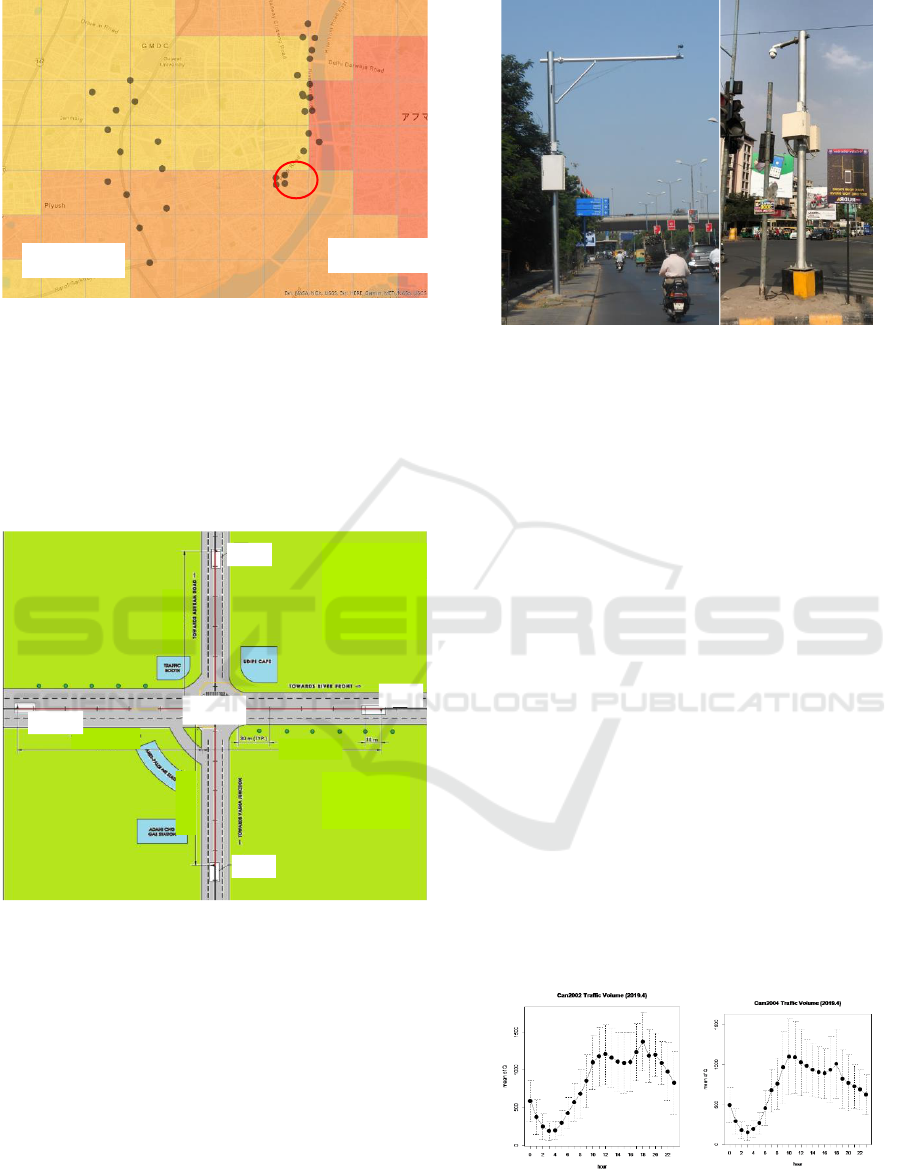
Figure 2: 1-Kilometer mesh with areal interpolation
population and traffic monitoring camera location (red
circle shows Paldi junction location and black dot marks are
traffic monitoring camera position) .
2.2 Paldi Junction
In Figure 3, it shows more detail location for traffic
monitoring cameras at Paldi junction.
Figure 3: There are four traffic monitoring cameras and
each traffic monitoring camera face to the centre of the
junction (Number shows traffic monitoring camera
location).
Each traffic monitoring camera monitors the number
of vehicles and average speed. For example, it
measures its traffic flow data of the vehicles which
come from North to the junction at Camera 2004. At
the centre of Paldi junction, there is a Surveillance
camera which can take high definition visual
condition and is remote controlled 360 degree. In
Figure 4, traffic monitoring camera and Surveillant
camera pictures are shown.
Figure 4: Traffic monitoring camera (left picture) and
Surveillant camera (right picture).
3 MESUREMENT & ANALYSIS
In this section, it shows actual traffic measurement
data and analysis at Paldi junction as Step 1. The
traffic data is collected by four traffic monitoring
cameras during April 2019 as an example data from
eight months monitoring. As for comparison
reference, another hourly measurement data is shown
in Appendix later (traffic volume and average vehicle
speed in January 2019. The trend of traffic volume is
similar with that in April).
3.1 Traffic Flow Data
As Step2, it focuses on the traffic flow especially
from North to South which is measured by Camera
2002 and 2004 as mention in the previous assumption.
The camera 2001 and 2002 data are shown in
Appendix. At first, Figure 5 shows the time-based
traffic volume at camera 2002 and 2004. The traffic
volume is one of traffic flow parameter and it is
defined as number of passing vehicle on the road per
hour.
(a) Traffic Volume at 2002 (b) Traffic Volume at 2004
Figure 5: Traffic Volume at camera 2002 and 2004.
167 meter
174 meter
169 meter
149 meter
A
B
C
D
E
A
B
C
D
E
2002
2001
2003
2004
Surveillanc
e camera
New town
Old town
Sabarmati River
Traffic Congestion “Gap” Analysis in India
483
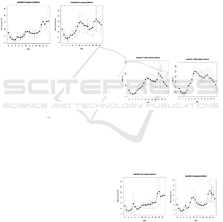
From Figure 5, traffic volume peak point is contrary
relevant in the morning 10:00 and evening 18:00. In
the morning, many vehicles go from North to South
for their business, then the traffic volume at 2004 is
larger than that of 2002. In the evening, it supposes
majority vehicles direction between 2002 and 2004 is
changed because of returning home.
In terms of traffic congestion, traffic occupancy is
capable to indicate its congestion rather than traffic
volume from previous study. In Figure 6, the
occupancy is shown.
(a) Occupancy at 2002 (b) Occupancy at 2004
Figure 6: Occupancy at camera 2002 and 2004.
As Step 3, it introduces the occupancy (OC)
which is also one of traffic flow parameter to analyse
quantitative traffic congestion. This is defined as
vehicle occupation percentage of road. (OC) is
calculated from traffic volume (q) and average
vehicle speed (v) by Equation (1) from traffic flow
theory.
𝑂𝐶 = 100 ×
𝑞
𝑣
× 𝑙
̅
(
%
)
(1)
where (q) is traffic volume, (v) is average vehicle
speed, and 𝑙
̅
is average vehicle length.
When it is compared between traffic volume trend
of Figure 5 and occupancy trend of Figure 6, traffic
volume does not always show its traffic congestion.
For example, from traffic monitoring camera 2004,
the highest peak of traffic volume occurs at 10:00, but
congested peak by occupancy occurs at 20:00. From
traffic monitoring experience, heavy traffic
congestion occurs over 20% occupancy. Therefore, in
case of traffic monitoring camera 2002, the traffic
volume in the morning is high but occupancy level is
less than 20%. This case is North and South traffic
movement. In terms of traffic flow direction, each
traffic monitoring camera faces towards the centre of
the junction. The traffic monitoring camera 2002
faces to the South and camera 2004 faces to the North.
Therefore, in the morning, the traffic volume from
North to South which means traffic volume of camera
2004 is higher than that of camera 2002. So, majority
of traffic flow moves from North to South. On the
other hand, the traffic volume from South to North in
the evening which means traffic volume of camera
2002 is higher than that of camera 2004. Majority of
traffic flow moves from South to North. The traffic
congestion occurs at 20:00.
From Figure 6, the evening traffic congestion
occurs at 20:00. But from Figure 5, the evening traffic
volume becomes peak at 18:00. There is two hours
“Gap” between each peak of occupancy and traffic
volume somehow. This “Gap” comes from the
balance between traffic volume and average vehicle
speed from Equation (1). This point is discussed in
the next section.
At the end of section, let’s check traffic flow from
east to west, which is based on measurement data
from traffic monitoring Camera No.2001 and 2003.
The traffic volume of both traffic monitoring
Camera 2001 and 2003 is shown in Figure 7.
(a) Traffic volume at 2001 (b) Traffic volume at 2003
Figure 7: Traffic volume at camera 2001 and 2003.
From east-west traffic volume observation in Figure 7,
▪ People movement from West to East in the
morning
▪ People movement from East to West in the
evening
In terms of occupancy at camera 2001 and 2003, it
shows hourly occupancy trend in Figure 8.
(a) Traffic Volume at 2001 (b) Traffic Volume at 2003
(a) Occupancy at 2001 (b) Occupancy at 2003
Figure 8: Traffic Occupancy at Camera 2001 and 2003.
VEHITS 2021 - 7th International Conference on Vehicle Technology and Intelligent Transport Systems
484
In this case, traffic congestion occurs at 20:00 in both
location. Here is congestion “Gap” between traffic
volume and occupancy again.
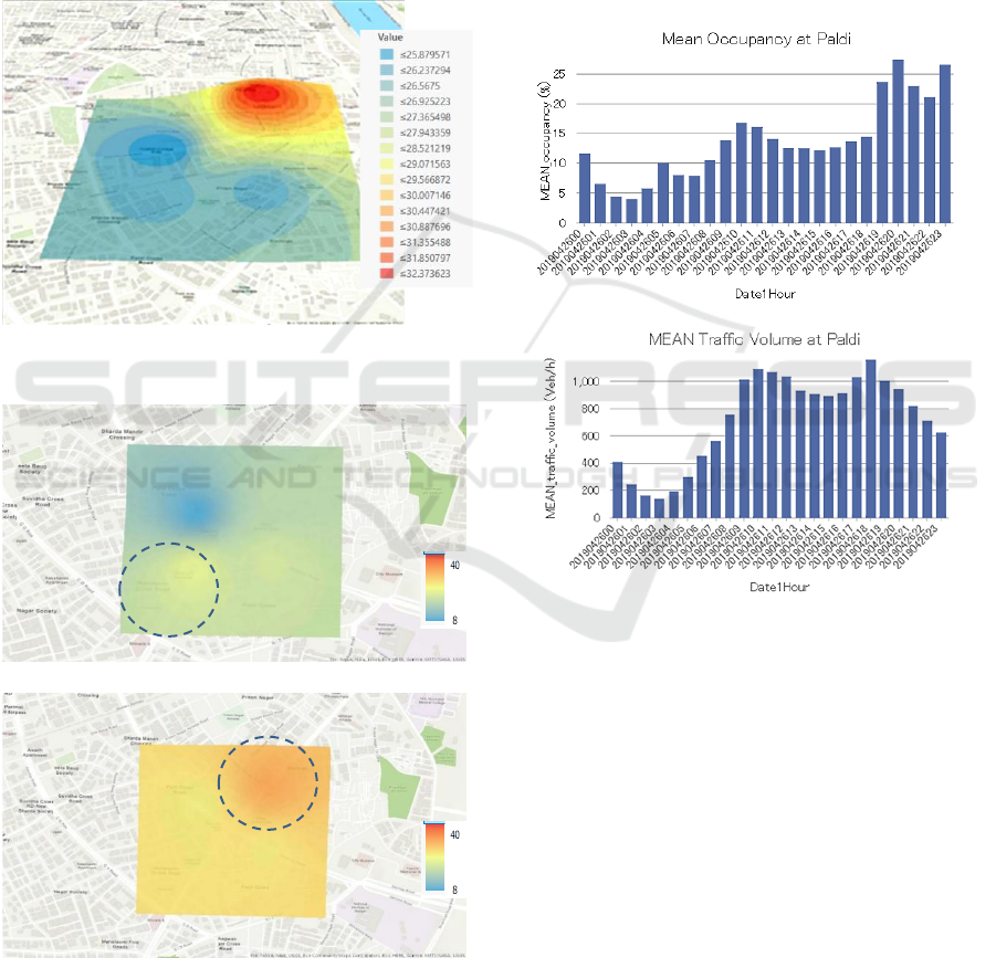
As Step 4 when it focuses on traffic congestion of
Paldi junction at 20:00, the three-dimensional
occupancy condition in Figure 9 provides its traffic
congestion image. In case of North and South, there
is heavy congestion in North. In case of East and West,
there are light congestions in both side. In Figure 10,
two GIS map at 10:00 and 20:00 in 26
th
of April are
shown as an example of traffic congestion situation.
Figure 9: Occupancy at Paldi junction in April 2019 20:00
(value shows the level of occupancy).
(a) Paldi junction occupancy at 10:00
(b) Paldi junction occupancy at 20:00
Figure 10: Occupancy at Paldi junction in 26
th
of April.
From Figure 9, it is clear that traffic congestion location is
different―south area in the morning and north area in the
evening.
3.2 Congestion Analysis
In the previous section, occupancy is one of
appropriate parameter for showing traffic congestion.
When we investigate the relationship between traffic
volume and occupancy from measurement, it shows
the summary of traffic volume and occupancy among
four traffic monitoring measurement on 26
th
of April
2019 in Figure 11. The number of traffic volume is
average among four traffic monitoring cameras and
its data unit is unified number of vehicles per hour per
lane.
(a) Traffic Volume at Paldi junction
(b) Occupancy at Paldi junction
Figure 11: Comparison between Traffic Volume and
Occupancy at Paldi junction on 26
th
of April 2019.
As mentioned earlier, there is congestion “Gap”
between traffic volume and occupancy peak. The
traffic volume peak occurs at 10:00 and 18:00 and the
Occupancy peak at 10:00 and 20:00. Time “Gap”
between traffic volume and occupancy in the evening
is two hours.
From this analysis result, traffic congestion is not
always happed under heavy traffic volume and there
must be some other reason behind. If heavy traffic
volume creates congestion, it should be happened in
the morning. But based on one-month traffic flow
observation, there is no traffic congestion in the
morning. And another important fact is why traffic
congestion “Gap” occurs in the evening, NOT in the
morning. These two points are decried in the next
Discussion section.
Traffic Congestion “Gap” Analysis in India
485

4 DISCUSSION
Let’s take one moment for traffic volume trend at
Paldi junction again. In Figure 12, it shows total four
traffic monitoring cameras time-based traffic volume
change in April 2019.
Figure 12: Accumulated Traffic Volume time-based change
at Paldi junction.
There are two peaks of traffic volume at 10:00 and
18:00. In case of occupancy, it shows total four traffic
monitoring cameras time-based traffic volume
change in April 2019 in Figure 13.
Figure 13: Accumulated Occupancy time-based change at
Paldi junction. From Figure 12, there are two peaks of
occupancy at 10:00 and 20:00. It is clear that there is
congestion “Gap” between traffic volume and
occupancy.
Table 2: Summary of Traffic Congestion “Gap”.
Cam
Congestion time
q max time
Congestion
“Gap” (hours)
No.
AM
PM
AM
PM
AM
PM
2001
―
20:00
10:00
18:00
―
2
2002
10:00
20:00
12:00
18:00
0
2
2003
10:00
20:00
10:00
18:00
0
2
2004
11:00
20:00
11:00
18:00
0
2
Table 2 summaries comparison between
congestion peek time from occupancy and traffic
volume peek time from traffic volume. There is two
hours congestion “Gap” of all location at Paldi
junction. In case of camera 2001, occupancy peek in
the morning occurs at 5:00. This situation comes from
no congestion of camera 2001 at 10:00 from Figure
13. Other camera 2002, 2003, and 2004 have third
peek of occupancy at 5:00 as well.
The Paldi junction environment is shown in
Figure 14 as an example of snapshot. In the junction,
there are traffic signal lights at each corner. And the
traffic signal control is used round lobbing access
with fixed time interval. There are several fixed time
interval selections and it is selected depend on its
traffic flow condition. This is typical Indian traffic
signal control method and it is necessary to have
detail traffic flow analysis related with traffic signal
control system in future.
Figure 14: Example Paldi junction traffic condition.
From the above all traffic flow measurement
observation long term and traffic flow analysis, it is
not clear why traffic congestion occurs in the evening,
NOT in the morning. We have several local traffic
officer’s discussions about Ahmedabad traffic
congestion issues and we found one of congestion
reason was transport behaviour as follows:
▪ Residents go straight to their office in the
morning by own private vehicles and then they
park their vehicle at certain regular parking
space.
▪ Some residents return straight to their home
after work but some go to shopping and or
restaurants for dinner in the evening. And there
is some difficulty to find parking space. In
general, there are not so many appropriate
parking area in India. Some people park along
the street when they are lucky to find the space.
If not, some people park their vehicles not
allowance space on the street, which makes
narrow the road width eventually.
▪ Local police officer does some time control its
traffic by manual because the fixed time interval
control does not effectively work for traffic
congestion, especially in the evening.
VEHITS 2021 - 7th International Conference on Vehicle Technology and Intelligent Transport Systems
486
In order to find out the reason for daily traffic
congestion in Ahmedabad, it is not only to have more
data but also check actual traffic condition time and
day such as investigation at 20:00 weekday. It is also
worth to have workshop among road management
group including traffic police and interviews to
residents. We also have other traffic monitoring
cameras s under the project and continue this traffic
management research by March 2022. As mentioned
earlier, the first city Metro is under development in
Ahmedabad and it will help to provide more
appropriate transportation choice to residents in near
future.
ACKNOWLEDGEMENTS
We appreciate support and collaboration from
Ahmedabad Municipal Corporation and local road
management authority as city traffic police and Smart
City Ahmedabad Development Ltd. This study
project was part of Program ID JPMJSA1606 of the
International Science and Technology Cooperation
Program (SATREPS) for global challenges in 2016.
REFERENCES
A.Salim, L.Vanajakshi, C.Subramanian, Estimation of
Average Space Headway under Heterogeneous Traffic
Conditions, International of Recent Trends in
Engineering and Technology, Vol. 3, No.5, 2010.
M.Goutham and B.Chanda, Introduction to the selection of
corridor and requirement, implementation of IHVS
(Intelligent Vehicle Highway System) In Hyderabad,
International Journal of Modern Engineering Research,
Vol.4, Iss.7, 2014, pp.49-54.
Population of India [Internet] 2020 Available From:
https://indiapopulation2019.com/population-of-ahme
dabad-2019.html [Accessed: 2020-08-21]
Registered number of vehicles Ahmedabad India FY 2006-
2017 Available From: https://www.statista.com/statis
tics/665754/total-number-of-vehicles-in-ahmedabad-
india/ [Accessed: 2020-08-21]
Ahmedabad Municipal Corporation Avilable From:
https://ahmedabadcity.gov.in/portal/jsp/Static_pages/i
ntroduction_of_amdavad.jsp [Accessed: 2020-08-21]
Tsuboi, T., 2018, Traffic Service Quantitative Analysis
Method under Developing Country, The 7th
International Conference on Advances in Computing,
Communications and Informatics (ICACCI).
Tsuboi, T., 2019, Traffic Congestion Visualization by
Traffic Parameters in India, 2nd International
Conference on Innovative Computing and
Communication (ICICC).
Tsuboi, T., 2019, Time Zone Impact for Traffic Flow
Analysis of Ahmedabad city in India, 4
th
International
Conference on Vehicle Technology and Intelligent
Transport System (VEHITS).
Tsuboi, T., 2020, New Traffic Congestion Analysis Method
in Developing Countries (India), 5
th
International
Conference on Vehicle Technology and Intelligent
Transport Systems (VEHITS).
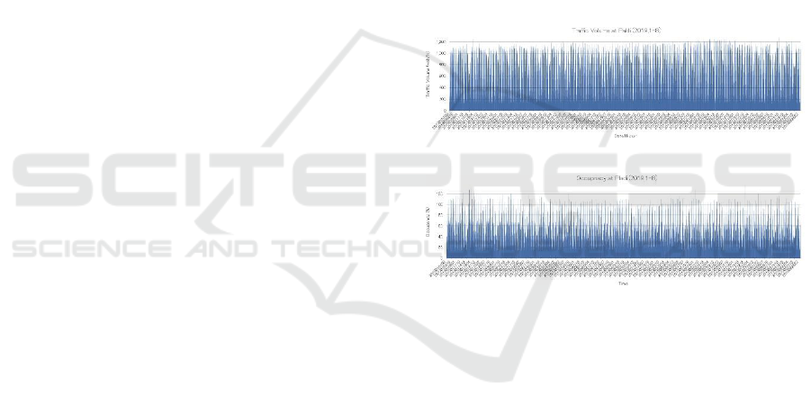
APPENDIX
Here is a reference data of traffic volume and
occupancy during 8 months from January to August
2019 in Figure A. The characteristics of traffic
volume and occupancy is based on all four traffic
monitoring camera and its value is used as average
data. Each characteristics are same trend by each
month, day, and time. Therefore, the analysis result
which is described in this paper is same result even if
it is taken other month or day.
(a) Traffic Volume trend during January to August 2019 at
Paldi junction
(b) Occupancy trend during January to August 2019 at Paldi
junction
Figure A: Long term Q and OC trend at Paldi junction.
Traffic Congestion “Gap” Analysis in India
487
