Point Cloud based Hierarchical Deep Odometry Estimation

Farzan Erlik Nowruzi

, Dhanvin Kolhatkar

, Prince Kapoor

and Robert Laganiere

1,2

School of Electrical Engineering and Computer Sciences, University of Ottawa, Canada

Sensorcortek Inc., Canada

Keywords:

Deep Learning, Lidar, Pointcloud, Odometry.

Abstract:

Processing point clouds using deep neural networks is still a challenging task. Most existing models focus on

object detection and registration with deep neural networks using point clouds. In this paper, we propose a

deep model that learns to estimate odometry in driving scenarios using point cloud data. The proposed model

consumes raw point clouds in order to extract frame-to-frame odometry estimation through a hierarchical

model architecture. Also, a local bundle adjustment variation of this model using LSTM layers is implemented.

These two approaches are comprehensively evaluated and are compared against the state-of-the-art.

1 INTRODUCTION

Autonomous vehicles should be able to operate in

known or unknown environments. In order to nav-

igate these environments, they have to be able to

precisely localize themselves. A major issue in lo-

calization and mapping is caused by the tight cou-

pling between these modules. We require highly pre-

cise maps for localization, while accurate localiza-

tion is required to create precise maps. This inter-

dependency has raised interest in methods that per-

form both tasks at the same time, termed Simultane-

ous Localization and Mapping (SLAM).

In an unknown environment, maps are not avail-

able for use as a priori of the environment model. A

localization module is needed to infer the position on

its own. One way to address this challenge is to es-

timate the amount of movement in between two in-

dividual observations and incrementally calculate the

location of a sensor in the coordinate frame of the ﬁrst

observation. This is termed odometry-based localiza-

tion. We propose to build a novel method to tackle

this problem by relying on the rich sensory data from

lidar in an unknown environment.

To achieve this, we utilize the power of deep neu-

ral models to build the backbone of the odometry

module. Deep models are not suited to perform tasks

such as localization using point cloud data out of the

box. In traditional methods, landmark extraction, data

association, ﬁltering and/or smoothing are used in a

pipeline to get the ﬁnal estimate. Our goal is to re-

place this pipeline with an end-to-end deep model.

Various traditional approaches (Zhang and Singh,

2014)(Chen et al., 2020) are proposed to perform

scan-to-scan matching to extract odometry data. The

majority of these models rely on using ICP and

RANSAC to extract the registration. The majority

of odometry estimation approaches utilize a temporal

ﬁltering stage that is classiﬁed as the Filtering or the

Bundle Adjustment. Filtering models summarize the

observations in compact representations. This makes

them lighter and faster than bundle adjustment meth-

ods that maintain a much larger set of observations

and constantly reﬁne their past and current predic-

tions.

Deep neural models have revolutionized many as-

pects of the computer vision ﬁeld (Simonyan and Zis-

serman, 2015)(Szegedy et al., 2016). Point-cloud pro-

cessing is one of the challenging scenarios that deep

models have a harder time expanding. This is due

to the complexity in the scale and the unordered na-

ture of the information representation in point-clouds.

(Zhou and Tuzel, 2018)(Qi et al., 2017a)(Qi et al.,

2017b)(Liu et al., 2019) have tackled this problem.

Many of these approaches are designed to address the

classiﬁcation and segmentation tasks on point-clouds.

A comprehensive review of these methods can be

found in (Guo et al., 2019). In this paper, we focus

on the application of deep models to the odometry-

based localization task. Using deep models for this

purpose is a fairly new ﬁeld and methods have not yet

matured enough. Unlike the current models that ex-

tract image-like representation of the data, our model

directly consumes point clouds. We employ models

112

Nowruzi, F., Kolhatkar, D., Kapoor, P. and Laganiere, R.

Point Cloud based Hierarchical Deep Odometry Estimation.

DOI: 10.5220/0010442901120121

In Proceedings of the 7th International Conference on Vehicle Technology and Intelligent Transport Systems (VEHITS 2021), pages 112-121

ISBN: 978-989-758-513-5

proposed for segmentation and classiﬁcation of point

cloud data as our feature extraction backbone. More

speciﬁcally, the input point-cloud data is processed

using Siamese PointNet++ layers (Qi et al., 2017b).

It follows the same architecture as Flownet3D (Liu

et al., 2019) in order to extract the correlation between

feature maps. The point-clouds used in Flownet3D

are captured from a single object and consist of fewer

points. The point-clouds used for odometry include a

much larger number of points, shifts, moving objects

and drastic changes in the environment. Flownet3D

uses up-convolutions to extract the 3D ﬂow between

two point-clouds. Instead, we pass the features maps

to fully connected layers to regress the rotation and

translation parameters.

2 RELATED WORK

Traditional visual localization methods such as LSD-

SLAM (Engel et al., 2014) and ORB-SLAM (Mur-

Artal et al., 2015) mainly rely on local features such

as SIFT (Lowe, 2004) and ORB (Rublee et al., 2011)

to detect the keypoints on camera images and track

them through multiple frames. Their lidar-based

counterparts, LOAM (Zhang and Singh, 2014) and

SLOAM (Chen et al., 2020), utilize a similar process-

ing framework with point-cloud data. The capabilities

of these models are always limited by the repeatabil-

ity of the hand-crafted features in consecutive frames.

One major issue in the odometry challenge is to

solve the data association or registration problem.

RANSAC (Hartley and Zisserman, 2003) like systems

are commonly used to rule out the outliers. Once the

data association is achieved, the transformation is es-

timated.

(Zhang and Singh, 2014) introduces Lidar based

Odometry and Mapping (LOAM), which is one of

the most prominent works in this ﬁeld. LOAM ex-

tracts key-points from lidar point-clouds and builds a

voxel grid-based map. They dynamically switch be-

tween frame-to-model and frame-to-frame operation

to simultaneously estimate odometry and build a map.

(Chen et al., 2020) builds on the idea of LOAM by re-

placing the key-points with semantic objects.

The use of learned features has been shown to pro-

vide better results in many computer vision tasks in

comparison to hand-crafted ones. Following the rev-

olution of deep learning in image processing, (Chen

et al., 2017) extracts deep learned features from im-

ages that are later used to perform the place recogni-

tion task. One of the early deep networks for camera

pose estimation is deﬁned in (Kendall et al., 2015)

and is termed PoseNet. It estimates the camera re-

localization parameters in 6 Degree-of-Freedom (6-

DoF) using a single image. In contrast with traditional

methods that rely on Bag of Words (BoW) (Fei-Fei

and Perona, 2005), this method only requires the net-

work weights and is highly scalable for place recog-

nition. However, as the network weights represent

a map, each new location will require a new train-

ing. (Brahmbhatt et al., 2018) increases the perfor-

mance of PoseNet by replacing the Euler angles with

the log of unit-quaternions and incorporating odom-

etry results from pre-existing methods. This param-

eterization of rotation only requires 3 values instead

of 4 parameters of quaternions and avoids over pa-

rameterization. On the other hand, (Cho et al., 2019)

shows that Euler angles are more stable than quater-

nion based loss in their study. (Sattler et al., 2018)

provides a comparison of visual localization methods

on multiple outdoor datasets with variable environ-

mental conditions.

In recent years, there is an increasing interest

in solving the odometry problem with deep learning

models. One of the ﬁrst works that directly tackles

the visual odometry challenge through an end-to-end

approach is proposed by (Wang et al., 2017). Odome-

try is estimated by utilizing a 9-layered convolutional

neural network with two LSTM layers at the end.

Processing point cloud data is very different than

processing images. Regularly, special tricks are ap-

plied on the point cloud to get an image-like represen-

tations and apply convolutional networks. (Li et al.,

2019) builds depth maps from lidar point-clouds and

uses it to extract surface normals. Using multi-task

learning, it tries to simultaneously estimate odometry

and build attention masks for geometrically consis-

tent locations through a Siamese model. Using their

combined loss function, they achieve comparable re-

sults to traditional approaches. (Cho et al., 2019) uti-

lizes two Siamese networks; one with surface normals

and the other with vertices. Features extracted from

both Siamese branches are summed and passed to an

odometry extraction network.

The deep neural models that take raw point-clouds

as input are categorized in two groups: Voxel-based

and Point-based methods. A voxel is a 3D partition in

the 3D point-cloud space.

Point-based approaches directly consume the

points in the cloud. These methods rely on local re-

gion extraction techniques and symmetric functions

to describe the selected points in each region. (Qi

et al., 2017a) introduces the idea of approximating

a symmetric function using a multi-layer perceptron

in order to process unordered point cloud data. Con-

volutional ﬁlters are used on these features to per-

form 3D shape classiﬁcation and object part segmen-

Point Cloud based Hierarchical Deep Odometry Estimation

113

tation. This work is expanded by PointNet++ (Qi

et al., 2017b) to better extract features from local

structures. This is achieved through the use of iter-

ative farthest point sampling and grouping of the un-

ordered points to hierarchically reduce their number

and only maintain a more abstract representation of

the original set.

Any deep learning approach that uses Siamese

model for odometry relies on a matching layer that

could be implemented in various forms. (Revaud

et al., 2016) introduces a new layer that hierarchically

extracts the image features for dense matching that is

used for ﬂow estimation. Flownet (Ilg et al., 2017)

convolves features of one Siamese branch against the

other and uses the results to explain the scene ﬂow.

3 DATA PRE-PROCESSING

We utilize KITTI an odometery dataset (Geiger et al.,

2012) in our experiments. In this section we describe

the pre-processing steps to prepare the input data to

our deep odometry model.

3.1 Label Extraction

The KITTI dataset employs global pose coordinates

on the local frame. Pose information is provided

from the view of the ﬁrst frame as the center of the

coordinate system. These, however, are not suit-

able labels for the frame-to-frame odometry estima-

tion task. Frame-to-frame pose transformations are

achieved through following formula:

i+1

= T

i,i+1

· X

i,i+1

= G

0,i+1

· G

−1

0,i

(1)

i,i+1

is the local transformation between two co-

ordinate centers X

and X

i+1

. G

0,i

and G

0,i+1

are the

global transformation from the ﬁrst frame (center of

the global coordinate frame) to the frames i and i + 1.

3.2 Point-cloud Sampling

The point-clouds in the KITTI dataset consist of 100k

points per frame. This is a huge set of points. Given

that lidar observations become less reliable at longer

distances, we remove any point farther than 50m from

the center in the x and z dimensions. There is still a

large number of points remaining after this step. To

reduce these points, we use the farthest point sam-

pling strategy (Eldar et al., 1997) to sample only 12k

and 6k points that are later used in our experiments.

Point-clouds collected in driving environments

usually contain a large amount of ground points,

which are not useful to extract motion information

and are usually discarded as a pre-processing step

(Ushani et al., 2017)(Liu et al., 2019). However,

ground as a ﬂat surface can provide cues regarding

the pitch and roll orientations of the vehicle, which is

valuable for the estimation of 6-DoF odometry. We

choose a 75% − 25% sampling ratio for non-ground

and ground points, in an attempt to balance the size of

the data and the accuracy of the system.

3.3 Dataset Augmentation

Another major issue with using deep learning models

for odometry results from the highly imbalanced na-

ture of the labels: the majority of roads are designed

as straight lines, with only a few turns made in long

drives. Deep learning models are highly dependent

on datasets being as complete as possible, which is

not the case in these scenarios.

On the dataset side, we employ over-sampling of

the minority labels to address this challenge. As a

result, models can learn the dynamics of the environ-

ment while assigning the required attention to minor-

ity transformations.

In 6-DoF motion, there are three rotation and three

translation parameters that need to be estimated. Ro-

tation components include α, β, and γ as the pitch,

yaw, and roll, and translation components consist of

motion in x, y, and z axes. There are various methods

that perform over-sampling - e.g. repetition, or Syn-

thetic Minority Over-Sampling Technique (Chawla

et al., 2002).

In order to achieve a more balanced dataset, we

use the repetition method based on the amount of

divergence from the average odometry value. To

augment the dataset, we ﬁrst calculate the average

and standard deviation for the rotation and translation

component norms individually. To decide on which

samples to use, we follow 3 rules:

• Translation: if x

< |µ

− aσ

| then augment with

T .

• Rotation: if x

< |µ

− aσ

| then augment with T .

• If both translation and rotation rules are satisﬁed

perform another augmentation run with x.

Subscripts r and t represent the rotation and trans-

lation components, respectively. x is the input norm,

µ is the average value, and σ is the standard deviation

for the corresponding input T . a is the ratio that is

used for the range interval.

Once a point pair is chosen to be repeated, number

VEHITS 2021 - 7th International Conference on Vehicle Technology and Intelligent Transport Systems

114

Figure 1: Histograms of the consecutive transformation pa-

rameters before and after data augmentation.

of copies N

is calculated using the following formula.

= d2

x−µ

a·σ

e (2)

D is a divisor value that explicitly controls the magni-

tude of the repetitions and is set to 4.

In this way, we add approximately 10000 samples

for rotation, 6000 samples for translation, and 2000

samples for both.

In the majority of driving scenarios, the cars are

in motion and are seldom stopped. To address this,

we repeat the identity transformation with a random

probability of 10% on the dataset. This results in the

addition of approximately 2000 samples to the train-

ing set.

Figure 1 compares the distribution of data points

before and after augmentation. The imbalance in spe-

ciﬁc components is not completely removed, but is

less than in the original dataset. This is especially the

case for yaw (b) and z components that have a major

effect on the accuracy of odometry. It is worth men-

tioning that, as all these components are correlated

with each other, completely removing the imbalance

only using this data is an impossibly challenging task.

4 MODEL ARCHITECTURE

4.1 Proposed Core Model

We rely on PointNet++ layers (Qi et al., 2017b) to

build our model. Similar to their model, we propose

a Siamese network that is able to regress the transfor-

mation between two point-clouds. Instead of passing

the whole point-cloud to a PointNet feature extrac-

tion layer, we divide the inputs into two groups; one

for ground points, and one for non-ground points. For

ground points, we only use a single PointNet layer

with a grouping distance threshold of 4 that outputs

400 points along with their descriptors. Descriptors

are generated using 3 consecutive multi-layer percep-

trons (MLP) of size (64, 96, 128). For non-ground

points, there are two layers that subsequently use

grouping distances of 0.5 and 1. 1500 points are pro-

duced in the ﬁrst layer and they are summarized to

800 points in the second layer. Both of these layers

use 3 MLPs where the ﬁrst one consists of (64,80, 96)

and the second one has layers of size (112, 128, 128).

The distance metric used to group ground points is

larger than the non-ground ones. This is due to the

harsher sampling performed on the ground points that

has resulted in larger distances between the points.

As the PointNet++ layers use farthest point sam-

pling internally, we keep the ground and non-ground

features separate for the feature extraction layer. The

ﬁnal outputs of ground and non-ground segments both

have a dimensionality of 128. Both feature maps are

concatenated along the points dimension building a

feature map of size 1200 × 128. At this stage, fea-

tures from each frame are passed to the ﬂow embed-

ding layer of (Liu et al., 2019). We use the cosine dis-

tance metric to correlate the features of each frame to

each other. For further future extraction in this layer,

we use the MLP with (128, 128, 128) width. Through

some experimentation, we found using nearest neigh-

bor with k = 10 gave the best results at this step. The

ﬁnal output shape of this layer is 1200 × 128.

Once the embedding between two frames is cal-

culated, we run another feature extraction layer with

radius of 1 and MLPs of size 128, 96, 64. This layer

is also responsible for reducing the number of feature

points that results in a feature map of shape 300 ×64.

All of the layers up to this stage include batch normal-

ization (Ioffe and Szegedy, 2015) after each convolu-

tion.

The resulting 2D feature map is ﬂattened and a

drop-out layer with keep probability of 0.6 is applied

on it. In order to extract the rotation and translation

parameters, we use two independent fully connected

layers of width 128 and 3.

The ﬁnal outputs of size 3 are concatenated to

build the 6-DoF Euler transformation parameters.

Figure 2 shows the architecture of this network.

4.2 Hierarchical Registration Model

In traditional literature (optimization or RANSAC

models) (Kitt et al., 2010)(Badino et al., 2013), an

odometry prediction is reﬁned quickly through mul-

tiple iterations. We argue that the same could be ap-

plied in the case of deep learning-based odometry es-

timation models. Inspired by a hierarchical homogra-

phy network (Nowruzi et al., 2017), we use multiple

layers of the same network to train on the residuals

of previous predictions. The new ground truth is cal-

culated by multiplying the ground truth from the pre-

Point Cloud based Hierarchical Deep Odometry Estimation

115

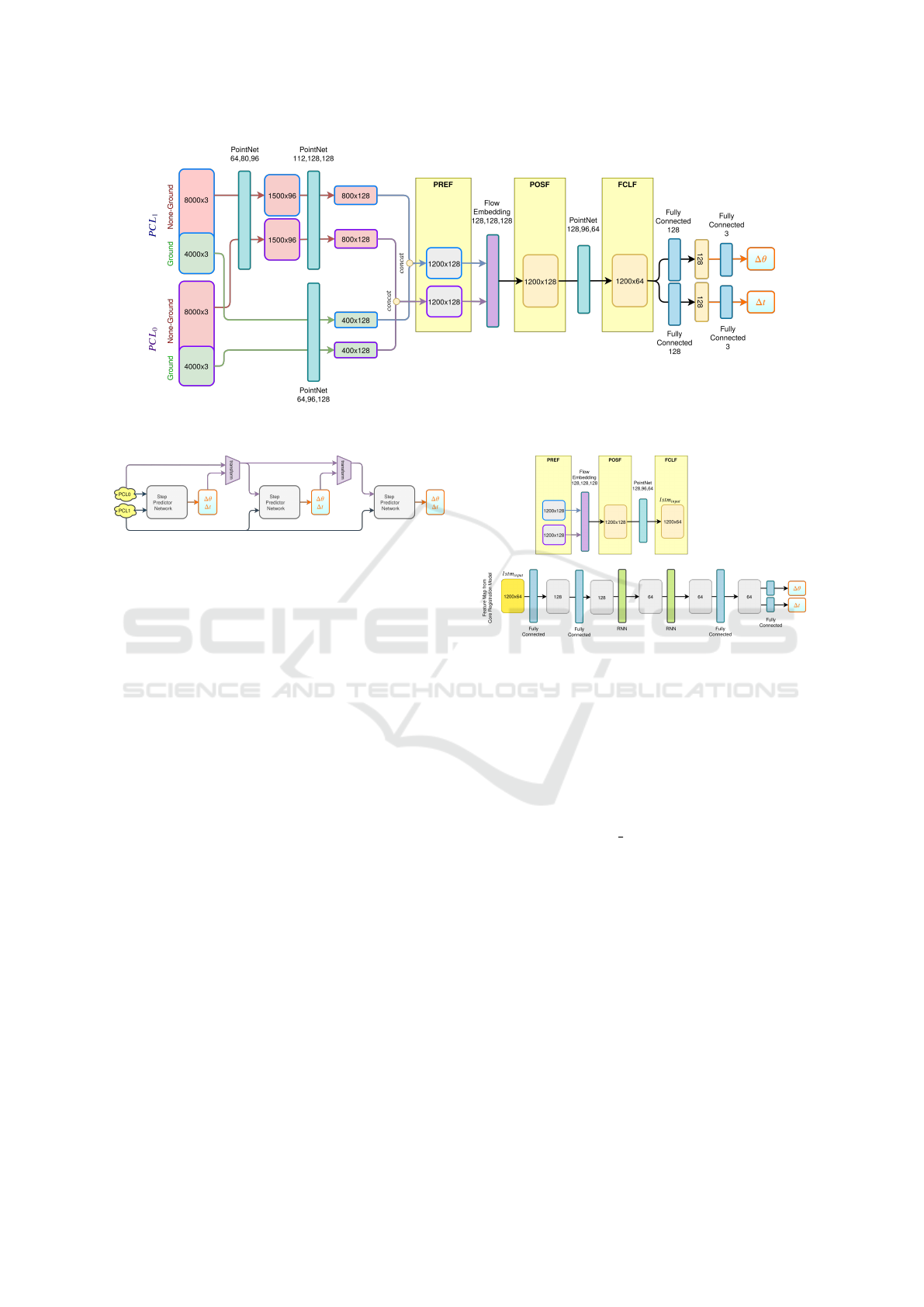
Figure 2: Proposed core registration model architecture to process two consecutive frames and extract transformation param-

eters in between them.

Figure 3: Progressive Prediction. In the ﬁrst iteration, ∆θ

and ∆t is estimated using PCL

and PCL

. The source point

cloud PCL

is transformed to PCL

. The residual trans-

formation between PCL

and X

is calculated and used to

estimate the next iteration of the model.

vious iteration by the inverse of its prediction. In this

way, each network reduces the dynamic range of error

from the previous models and successively achieves a

better result. Figure 3 shows this process.

The higher accuracy comes with the cost of in-

creased train and test times. The key element in this

approach is to keep the computational complexity as

low as possible for each module in order to satisfy

real-time processing requirements for the odometry

task.

4.3 Temporal Filtering

The goal of the odometry model is to smooth the ef-

fect of errors caused by the registration network. Our

proposed model requires a large amount of memory

due to its mid-level feature representation. Adding

the memory requirements that the temporal model im-

poses, training quickly becomes a challenge for the

system. Furthermore, training the core registration

network is already a difﬁcult task. Extra parametriza-

tion from the LSTM model makes an already difﬁcult

task an even more challenging one.

To alleviate these issues we propose a two stage

training approach that breaks the initial feature extrac-

tor and the temporal ﬁlter into two disjoint models.

Once the core registration network is trained, mid-

Figure 4: Temporal model along with the three different

input levels. FCLF is the natural input state of the temporal

model. PREF and POSF require additional layers from the

registration model to be included and re-learned inside the

temporal model.

level features are extracted and used as inputs to train

the temporal model.

The base of our proposed temporal model consists

of two fully connected layers of width 64 and 128. It

is followed by two bidirectional LSTM with 64 hid-

den layers with a soft sign activation function. The

output of the LSTM is fed to a fully connected layer

with a size of 64. Finally, in the output layer, we

have two fully connected networks with 3 nodes each

that estimate the rotation and translation, individually.

Figure 4 shows this model.

We employ drop-out and batch-normalization af-

ter each layer. For the LSTM model, a temporal win-

dow of 5 frames is utilized.

4.4 Loss Function

As explained in Section 3, the odometry labels suffer

from data imbalance problem. The majority of the in-

stances in the dataset follow a straight line, with only

a few of them constituting the turns. To tackle these

VEHITS 2021 - 7th International Conference on Vehicle Technology and Intelligent Transport Systems

116

challenges, we incorporate measures in our loss func-

tion.

Using the naive L2-norm diminishes the effect of

instances with larger errors, as most of the batches

result in smaller errors. It is required to make the

model more sensitive towards larger errors. This

is achieved through the use of online-hard-example-

mining (OHEM) loss (Shrivastava et al., 2016). In

OHEM, only the top k samples with highest loss val-

ues are used to calculate the ﬁnal loss. However, once

this value is set it does not change during the train.

This could result in a training session that has high

ﬂuctuations in loss values. To address this, we im-

plement an adaptive version of OHEM loss, that in-

creases the number of top k after certain epochs. The

model initially focuses on the hardest examples, be-

fore its attention shifts towards all of the examples.

This provides the hardest examples that are less fre-

quent with a chance to drive the network towards the

global minimum.

Another aspect of the loss function is to analyze

the effects of errors in each component of the label.

Rotation and translation components are separately

extracted from the model. To enable the model’s ca-

pability of adapting to each component, instead of us-

ing the naive approach, we employ a weighting mech-

anism. To introduce uncertainty in our loss function,

we consider the log of normal distribution and phrase

it as a minimization problem. In odometry, there are

6 parameters to be learnt that represent two compo-

nents. We use the same weight for parameters related

to each component. In order to practically implement

this loss function, we replace the standard deviation

σ of normal distribution with exp(w) that ensures the

learned uncertainty is represented by a positive value.

This results in the following ﬁnal loss function.

=exp(−w

)kx

− ˆx

k + w

exp(−w

)kx

− ˆx

k + w

(3)

and x

are predicted translation and rotation

variables. ˆx

and ˆx

deﬁne the ground-truth. w

and

are the trainable weighting parameters, and l

de-

ﬁnes the ﬁnal loss.

5 EXPERIMENTS

Estimating 6-DoF odometry using point-clouds is a

challenging task. All the points are down sampled

as described in section 3. We ﬁrst use the registra-

tion model to extract the transformation between two

frames. This could be repeated for all the point-cloud

pairs to generate the odometry trace. However, the

Figure 5: Estimated odometry trace for KITTI sequences

using 8k4k comp model. Sequences 00-08 are used to train,

and sequences 09-10 are used as test data for the model.

additive nature of the noise quickly drifts the trace

away from the ground truth. Due to this fact, there is

no single metric that can explain all the various fail-

ures in the system. We evaluate various aspects of

the model using KITTI odometry metrics; Absolute

Trajectory Error (ATE), Sequence Translation Drift

Percentage, Sequence Rotation error per 100 meters,

Relative Rotation Error (RRE) and Relative Transla-

tion Error (RTE)

RTE and RRE are the most important metrics as

they evaluate the effectiveness of model for frame-to-

frame estimation, independent of the trajectory. This

is the main target that model is trained for.

5.1 Hierarchical Model

In this section we evaluate the performance of the hi-

erarchical model acronymed as 8k4k comp. Figure

5 shows the trajectories of various training iterations

and Figure 6 presents their error metrics. As expected,

estimates of the second iteration are far superior to

the ﬁrst iteration. The third iteration reduces the error

further but the reduction rate is smaller than the previ-

ous iteration. This is due to the fact that after certain

point, the learning process will plateau as the amount

of information to learn is much smaller. The trend is

clearly visible in RTE and RRE metrics.

5.2 Temporal Model

Another way to increase the accuracy of odometry is

by employing temporal features. However, training

the frame-to-frame estimation model requires a sig-

niﬁcant amount of system resources. Adding LSTM

on top of that model will dramatically increase these

requirements. In such cases, it is common to use

a pre-trained feature extraction network and provide

mid-level features as inputs to an LSTM model. Fol-

lowing this idea, we evaluate three features maps

taken from various layers of our trained model.

• Feature maps immediately before the ﬂow embed-

ding layer (PREF).

Point Cloud based Hierarchical Deep Odometry Estimation

117

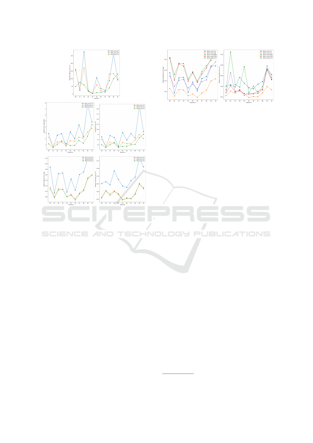
Figure 6: Comparison of various iterations of the proposed

model.

• Feature maps immediately after the ﬂow embed-

ding layer (POSF).

• Feature maps prior to the fully connected layers in

the feature extraction network (FCLF).

PREF is the earliest level of features among the

three. This model requires the largest temporal model

as the ﬂow embedding and the feature extraction lay-

ers from the original model are retrained in temporal

model.

To reduce the complexity further, POSF features

are used. This is achieved by employing features af-

ter the ﬂow embedding layer. However, a point-cloud

feature extractor needs to be present in the LSTM.

Finally, FCLF is the smallest feature map. Most

of the ﬂow matching and feature extraction work is

completed and only the fully connected model is left

for the LSTM model.

FCLF features are outperforming both PREF and

POSF features. This is the objective that is used to

train the frame-to-frame registration model. FCLF

mimics the registration model rather than learning

temporal features as the provided features are much

less informative compared to PREF and POSF.

Figure 7 shows the results of these comparisons.

It is seen that the usage of mid-level features is not as

Figure 7: Comparison of the performance of the temporal

model.

fruitful as using a second iteration. In some cases the

results are worse than the original feature extraction

model that is all attributed to the dividing the training

process into two parts.

5.3 Comparison to the State-of-the-Art

In this group of experiments, we compare the pro-

posed model to the state-of-the-art. Table 1 com-

pares various models in terms of sequence translation

drift percentage and mean sequence rotation error for

lengths of [100, 800]m. Please note that the results for

LOAM (Zhang and Singh, 2014), ICP

reported

are taken

from (Li et al., 2019).

LOAM (Zhang and Singh, 2014) is one of the

benchmarks in this ﬁeld. It clearly outperforms all

of the deep methods in the comparison. One main

reason for that is the feature extraction back-bone net-

work. In our work, we relied on PointNet++ (Qi et al.,

2017b) features. Both LO-Net (Li et al., 2019) and

DeepLO (Cho et al., 2019) use 2D depth and surface

models such as vertex and normal representations.

This way, they completely avoid the usage of 3D data

for feature extraction. This trend is also visible across

the ﬁeld as 2D feature extraction models are more ad-

vanced than their 3D counterparts. However, there is

a growing interest regarding the 3D feature extraction

methods (Wang et al., 2019)(Wu et al., 2019) that can

enhance the performance of deep odometry estima-

tion with 3D point clouds.

It is clearly seen that DeepLO (Cho et al., 2019)

is over-ﬁtting to the training set. Our model is also

suffering from such a phenomenon, but the scale of

over-ﬁtting is much lower. One reason for this is the

size of our model compared to the size of the input

dataset. Using PointNet++ layers results in large net-

works that require a large amount of data. LO-Net (Li

et al., 2019) addresses this problem by utilizing a 2D-

based feature extraction network (Zhou et al., 2017).

We use an implementation of the ICP algorithm from

the Open3D library

. In our implementation we use

http://www.open3d.org/

VEHITS 2021 - 7th International Conference on Vehicle Technology and Intelligent Transport Systems

118

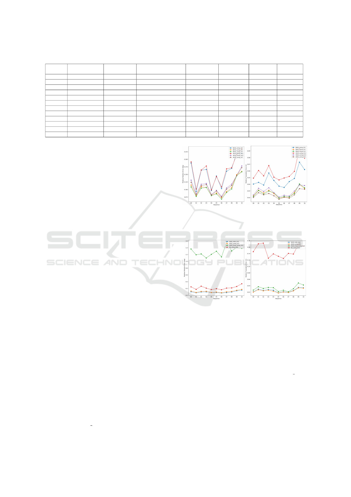
Table 1: Sequence translation drift percentage and mean sequence rotation error for the lengths of [100, 800]m.

DeepLO LO-Net LOAM ICP

reported

(Cho et al., 2019) (Li et al., 2019) (Zhang and Singh, 2014) (Li et al., 2019) ICP Ours Ours+ICP

Sequence t

rel

00 0.32 0.12 1.47 0.72 1.10 0.53 6.88 2.99 32.14 13.4 3.41 1.48 2.38 1.08

01 0.16 0.05 1.36 0.47 2.79 0.55 11.21 2.58 3.52 1.14 1.55 0.68 2.01 0.60

02 0.15 0.05 1.52 0.71 1.54 0.55 8.21 3.39 22.64 7.02 3.35 1.40 2.81 1.27

03 0.04 0.01 1.03 0.66 1.13 0.65 11.07 5.05 37.30 4.76 6.13 2.07 5.68 1.65

04 0.01 0.01 0.51 0.65 1.45 0.50 6.64 4.02 2.91 1.34 2.04 1.51 1.65 1.21

05 0.11 0.07 1.04 0.69 0.75 0.38 3.97 1.93 56.91 19.93 2.17 1.09 1.74 0.99

06 0.03 0.07 0.71 0.50 0.72 0.39 1.95 1.59 29.30 6.93 2.47 1.10 1.66 0.89

07 0.08 0.05 1.70 0.89 0.69 0.50 5.17 3.35 42.01 28.80 3.62 1.91 1.23 0.92

08 0.09 0.04 2.12 0.77 1.18 0.44 10.04 4.93 36.58 12.36 3.61 1.61 2.74 1.29

∗

13.35 4.45 1.37 0.58 1.20 0.48 6.93 2.89 36.54 12.82 8.26 3.11 2.69 1.57

∗

5.83 3.53 1.80 0.93 1.51 0.57 8.91 4.74 28.54 6.48 11.19 5.65 6.22 2.33

the sub-sampled point-clouds. This results in a signif-

icant drop in performance in comparison to the results

of ICP

reported

(Li et al., 2019) that use the full point

cloud. However, using the full point cloud data entails

a large computational complexity burden. The sub-

sampling stage that is used to reduce the computa-

tional complexity is another aspect that affects the es-

timation performance of our model. The same points

are not always chosen to represent the same static ob-

jects. This inherently adds noise to our dataset. We

further explore using ICP as a ﬁnal step on our es-

timates that signiﬁcantly improves the performance.

This is an expected outcome, as the complexity of the

residual problem to solve for ICP at this stage is less

than the original one. Hence, it can easily ﬁnd the

corresponding points and estimate better registration

parameters.

5.4 Input Dimensionality

We evaluate the performance of the models with 12k

and 6k input points. 8k4k represents the 8k and 4k di-

vision between non-ground and ground points. Sim-

ilarly, 4k2k corresponds to 4k ground and 2k non-

ground point sampling. Extra points only help in

providing better descriptors at the ﬁrst layer where

the ﬁrst sampling function in the network is called.

This results in better performance of the model, espe-

cially in the ﬁrst iteration where the disparity between

matching points in two frames is much larger. How-

ever, the difference diminishes in the second and third

iterations. This entails that by employing a hierarchi-

cal model we could reduce the complexity of the input

point cloud by using coarser 3D point clouds. Results

of this comparison are shown in Figure 8.

5.5 Sampling Comparison

To better understand the importance of separately

sampling ground and non-ground points, we train

the same model (6k comp) with 6k globally sampled

Figure 8: Input point cloud dimensionality analysis. 8k4k

indicates 8k non-ground and 4k ground points in the input

cloud. 4k2k uses 4k non-ground and 2k ground points in

the input cloud.

Figure 9: Comparative results for various ablation stud-

ies.4k2k uses 4k non-ground and 2k ground points as its

input. 6k indicates that 6k points are globally sampled with-

out any distinction between ground and non-ground points.

comp uses one weight for the rotation component and one

weight for the translation component in the loss function.

indiv uses individual weights for each parameter in the pose.

tmat indicates that the rotation matrix is used instead of nor-

malized Euler angles to calculate the loss.

points from the point cloud. We train this model in

hierarchical manner and compare it to the 4k2k comp

model that employs 4k non-ground and 2k ground

input points. As it is shown in Figure 9, sampling

without distinction between ground and non-ground

points results in far worse performance. This is due

the large number of ground points in the point cloud

that provide much less information regarding transla-

tion and orientation of the sensor in comparison to the

Point Cloud based Hierarchical Deep Odometry Estimation

119

non-ground points.

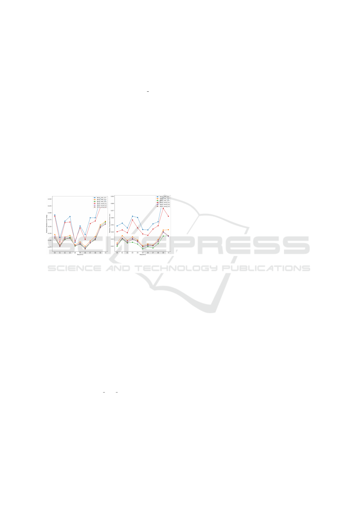
5.6 Loss Comparison

The proposed model employs weighted l2 norm loss

on Euler angles and translation parameters. The loss

function utilizing 2 weights for each rotation and

translation components is indicated with comp, while

the indiv represents the usage of individual weights

for each transformation parameter.

Figure 10 shows comparative results of this ex-

periment. We observe that in the ﬁrst two iterations,

component based weighting provides better results.

However, in the third iteration, individual weighting

achieves comparable results to the component based

function. It is worth mentioning that the scale of re-

duction in error between iteration 2 and 3 is small,

and the majority of the error reduction is achieved in

the ﬁrst 2 iterations.

Figure 10: Comparative results over various iterations for

comp vs indiv weighting scheme in loss function. comp

uses one weight for rotation component and one weight for

translation component in the loss function. indiv uses indi-

vidual weights for each parameter in the pose.

5.7 Label Representation

Normalized Euler angles are used as the primary la-

bels along with normalized translation parameters in

our experiments. Normalization is utilized in order to

remove the scaling effects for various parameters in

calculation of the L2-norm. To validate our decision,

we compare our choice of label representation to the

transformation matrix representation with 12 parame-

ters (3 × 3 rotation and 3 translation). We employ the

component-based weighting on rotation and transla-

tion components of this representation. The trained

model is shown as 4k2k tmat comp in Figure 9. Re-

sults show that normalized Euler angles are a much

better representation than the 3 × 3 rotation matrix,

which is an over-parameterized representation of the

rotation.

6 CONCLUSION

In this paper, we have proposed a methodology to use

deep neural networks to estimate odometry based on

3D point clouds. We have proposed a data augmenta-

tion mechanism along with measures incorporated in

the loss function to estimate the frame-to-frame trans-

formation parameters. The proposed model success-

fully reduces the error in consecutive iterations. Fur-

thermore, we have evaluated the usage of pre-trained

feature maps for training temporal models. Our re-

sults are comparable to the state-of-the-art. We argue

that the extracted features from the 3D point clouds

are not descriptive enough for this task. 3D point-

cloud-based deep learning is still a new ﬁeld and 3D

deep feature extraction techniques have not matured

as much as their 2D image-based counterparts.

REFERENCES

Badino, H., Yamamoto, A., and Kanade, T. (2013). Vi-

sual odometry by multi-frame feature integration. In

Proceedings of the IEEE International Conference on

Computer Vision Workshops.

Brahmbhatt, S., Gu, J., Kim, K., Hays, J., and Kautz, J.

(2018). Geometry-aware learning of maps for camera

localization. In Proceedings of the IEEE Conference

on Computer Vision and Pattern Recognition.

Chawla, N. V., Bowyer, K. W., Hall, L. O., and Kegelmeyer,

W. P. (2002). Smote: synthetic minority over-

sampling technique. Journal of artiﬁcial intelligence

research.

Chen, S. W., Nardari, G. V., Lee, E. S., Qu, C., Liu, X.,

Romero, R. A. F., and Kumar, V. (2020). Sloam: Se-

mantic lidar odometry and mapping for forest inven-

tory. IEEE Robotics and Automation Letters.

Chen, Z., Jacobson, A., S

underhauf, N., Upcroft, B., Liu,

L., Shen, C., Reid, I., and Milford, M. (2017). Deep

learning features at scale for visual place recognition.

In Robotics and Automation (ICRA), 2017 IEEE Inter-

national Conference on. IEEE.

Cho, Y., Kim, G., and Kim, A. (2019). Deeplo:

Geometry-aware deep lidar odometry. arXiv preprint

arXiv:1902.10562.

Eldar, Y., Lindenbaum, M., Porat, M., and Zeevi, Y. Y.

(1997). The farthest point strategy for progressive im-

age sampling. IEEE Transactions on Image Process-

ing.

Engel, J., Sch

ops, T., and Cremers, D. (2014). Lsd-slam:

Large-scale direct monocular slam. In European Con-

ference on Computer Vision. Springer.

Fei-Fei, L. and Perona, P. (2005). A bayesian hierarchical

model for learning natural scene categories. In Com-

puter Vision and Pattern Recognition, 2005. CVPR

2005. IEEE Computer Society Conference on. IEEE.

Geiger, A., Lenz, P., and Urtasun, R. (2012). Are we ready

for autonomous driving? the kitti vision benchmark

VEHITS 2021 - 7th International Conference on Vehicle Technology and Intelligent Transport Systems

120

suite. In Conference on Computer Vision and Pattern

Recognition (CVPR).

Guo, Y., Wang, H., Hu, Q., Liu, H., Liu, L., and Ben-

namoun, M. (2019). Deep learning for 3d point

clouds: A survey. arXiv preprint arXiv:1912.12033.

Hartley, R. and Zisserman, A. (2003). Multiple view geom-

etry in computer vision. In Multiple view geometry in

computer vision. Cambridge university press.

Ilg, E., Mayer, N., Saikia, T., Keuper, M., Dosovitskiy, A.,

and Brox, T. (2017). Flownet 2.0: Evolution of optical

ﬂow estimation with deep networks. In Proceedings of

the IEEE conference on computer vision and pattern

recognition.

Ioffe, S. and Szegedy, C. (2015). Batch normalization: Ac-

celerating deep network training by reducing internal

covariate shift. In Proceedings of the 32nd Interna-

tional Conference on Machine Learning, Proceedings

of Machine Learning Research. PMLR.

Kendall, A., Grimes, M., and Cipolla, R. (2015). Posenet: A

convolutional network for real-time 6-dof camera re-

localization. In Proceedings of the IEEE international

conference on computer vision.

Kitt, B., Geiger, A., and Lategahn, H. (2010). Visual odom-

etry based on stereo image sequences with ransac-

based outlier rejection scheme. In 2010 ieee intelli-

gent vehicles symposium. IEEE.

Li, Q., Chen, S., Wang, C., Li, X., Wen, C., Cheng, M., and

Li, J. (2019). Lo-net: Deep real-time lidar odometry.

In Proceedings of the IEEE Conference on Computer

Vision and Pattern Recognition.

Liu, X., Qi, C. R., and Guibas, L. J. (2019). Flownet3d:

Learning scene ﬂow in 3d point clouds. In Proceed-

ings of the IEEE Conference on Computer Vision and

Pattern Recognition.

Lowe, D. G. (2004). Distinctive image features from scale-

invariant keypoints. International journal of computer

vision.

Mur-Artal, R., Montiel, J. M. M., and Tardos, J. D. (2015).

Orb-slam: a versatile and accurate monocular slam

system. IEEE Transactions on Robotics.

Nowruzi, F. E., Japkowicz, N., and Laganiere, R. (2017).

Homography estimation from image pairs with hier-

archical convolutional networks. In Computer Vision

Workshop (ICCVW), 2017 IEEE International Confer-

ence on. IEEE.

Qi, C. R., Su, H., Mo, K., and Guibas, L. J. (2017a). Point-

net: Deep learning on point sets for 3d classiﬁcation

and segmentation. In Proceedings of the IEEE confer-

ence on computer vision and pattern recognition.

Qi, C. R., Yi, L., Su, H., and Guibas, L. J. (2017b). Point-

net++: Deep hierarchical feature learning on point sets

in a metric space. In Advances in neural information

processing systems.

Revaud, J., Weinzaepfel, P., Harchaoui, Z., and Schmid,

C. (2016). Deepmatching: Hierarchical deformable

dense matching. International Journal of Computer

Vision, 120(3).

Rublee, E., Rabaud, V., Konolige, K., and Bradski, G.

(2011). Orb: An efﬁcient alternative to sift or surf.

In Computer Vision (ICCV), 2011 IEEE international

conference on.

Sattler, T., Maddern, W., Toft, C., Torii, A., Hammarstrand,

L., Stenborg, E., Safari, D., Okutomi, M., Pollefeys,

M., Sivic, J., et al. (2018). Benchmarking 6dof out-

door visual localization in changing conditions. In

Proc. CVPR, volume 1.

Shrivastava, A., Gupta, A., and Girshick, R. (2016). Train-

ing region-based object detectors with online hard ex-

ample mining. In Proceedings of the IEEE conference

on computer vision and pattern recognition.

Simonyan, K. and Zisserman, A. (2015). Very deep con-

volutional networks for large-scale image recognition.

In International Conference on Learning Representa-

tions.

Szegedy, C., Vanhoucke, V., Ioffe, S., Shlens, J., and Wo-

jna, Z. (2016). Rethinking the inception architecture

for computer vision. In Proceedings of the IEEE con-

ference on computer vision and pattern recognition.

Ushani, A. K., Wolcott, R. W., Walls, J. M., and Eustice,

R. M. (2017). A learning approach for real-time tem-

poral scene ﬂow estimation from lidar data. In 2017

IEEE International Conference on Robotics and Au-

tomation (ICRA). IEEE.

Wang, S., Clark, R., Wen, H., and Trigoni, N. (2017).

Deepvo: Towards end-to-end visual odometry with

deep recurrent convolutional neural networks. CoRR.

Wang, Y., Sun, Y., Liu, Z., Sarma, S. E., Bronstein, M. M.,

and Solomon, J. M. (2019). Dynamic graph cnn

for learning on point clouds. ACM Transactions on

Graphics (TOG).

Wu, W., Qi, Z., and Fuxin, L. (2019). Pointconv: Deep

convolutional networks on 3d point clouds. In Pro-

ceedings of the IEEE Conference on Computer Vision

and Pattern Recognition.

Zhang, J. and Singh, S. (2014). Loam: Lidar odometry

and mapping in real-time. In Robotics: Science and

Systems.

Zhou, T., Brown, M., Snavely, N., and Lowe, D. G. (2017).

Unsupervised learning of depth and ego-motion from

video. In Proceedings of the IEEE Conference on

Computer Vision and Pattern Recognition.

Zhou, Y. and Tuzel, O. (2018). Voxelnet: End-to-end learn-

ing for point cloud based 3d object detection. In Pro-

ceedings of the IEEE Conference on Computer Vision

and Pattern Recognition.

Point Cloud based Hierarchical Deep Odometry Estimation

121