
Exploring Differential Privacy in Practice
Davi Grossi Hasuda and Juliana de Melo Bezerra
Computer Science Department, ITA, S
˜
ao Jos
´
e dos Campos, Brazil
Keywords:
Privacy, Differential Privacy, Classification Algorithms, Accuracy, Data Analysis.
Abstract:
Every day an unimaginable amount of data is collected from Internet users. All this data is essential for
designing, improving and suggesting products and services. In this frenzy of capturing data, privacy is often
put at risk. Therefore, there is a need for considering together capturing relevant data and preserving the
privacy of each person. Differential Privacy is a method that adds noise in data in a way to keep privacy. Here
we investigate Differential Privacy in practice, aiming to understand how to apply it and how it can affect data
analysis. We conduct experiments with four classification techniques (including Decision Tree, N
¨
aive Bayes,
MLP and SVM) by varying privacy degree in order to analyze their accuracy. Our initial results show that low
noise guarantees high accuracy; larger data size is not always better in the presence of noise; and noise in the
target does not necessary disrupt accuracy.
1 INTRODUCTION
It is noticeable that data is an important asset of the
globalized world. Every moment, a lot of new data
is being generated by users of the Internet worldwide,
which is actually useful for many companies that in-
vest in storing and processing all the data they can col-
lect (World, 2018). Amazon.com, for instance, devel-
oped its Recommender System by searching for users
with similar interests, and made suggestions based on
this similarity (Smith and Linden, 2017). Generally,
for companies to understand how the user experience
is evolving with the product or service, they have to
collect user data (Havir, 2017). Another important
factor of the globalized world is the fact that some of
this data is used to train neural networks, and very
often this training requires a great amount of data.
Face ID, for example, the Apple’s system to recog-
nize someone’s face and authenticate based on that,
took over 1 billion images to train its neural network
(Apple, 2017b).
In the midst of the frenzy of collecting data,
many times privacy is jeopardized (Buffered.com,
2017). One of the most emblematic case was the
scandal involving Facebook and Cambridge Analyt-
ica (Granville, 2018), where Facebook provided the
data and Cambridge Analytica used it improperly to
influence the presidential run in the United States.
Another example was with Tanium, a cybersecurity
startup, that exposed the network of a client without
permission (Winkler, 2017). Concerned about these
privacy scandals, there are some efforts emerging in
order to preserve privacy. GDPR, for instance, is the
General Data Protection Regulation (GDPR, 2018)
from the European Union that rewrites how data shar-
ing must work on the Internet. GDPR describes con-
straints and rules when accessing and sharing user
data. Another effort, which is the focus of our pa-
per, is Differential Privacy (DP)(Dwork, 2006). DP
establishes constraints to algorithms that concentrate
data in a statistical database. Such constraints limit
the privacy impact on individuals whose data is in the
database.
Simple anonymization processes can be very inef-
fective for assuring privacy. For example, there is the
case of 2006 Netflix Prize, a competition promoted
by Netflix where competitors must develop an algo-
rithm to predict ratings from users. For that, Netflix
shared a dataset with over 100 million ratings by over
480 thousand users. All the names were removed, and
some fake ratings were added. But as shown later,
it was not enough, since a de-anonymization process
was possible by comparing the Netflix dataset with an
IMDb dataset (Dwork and Roth, 2014). So, the pro-
cess that privatize data must be linkage attack-proof.
Besides, it must not compromise the final result of
machine learning algorithms and statistical studies
where they are used. It means that, after the privatiza-
tion process, it is expected that the data is still useful
(Abadi et al., 2016). Fortunately, Differential Privacy
already takes that in count. Moreover, DP provides a
way of measuring privacy (Dwork and Roth, 2014).
Hasuda, D. and Bezerra, J.
Exploring Differential Privacy in Practice.
DOI: 10.5220/0010440408770884
In Proceedings of the 23rd International Conference on Enterprise Information Systems (ICEIS 2021) - Volume 1, pages 877-884
ISBN: 978-989-758-509-8
Copyright
c
2021 by SCITEPRESS – Science and Technology Publications, Lda. All rights reserved
877

Most of the papers regarding DP focus on theory,
considering definition, foundations and algorithms re-
lated to DP (Dwork, 2006; Dwork and Roth, 2014;
Dwork et al., 2006; Dwork and Rothblum, 2016).
(Jain and Thakurta, 2014) propose a privacy preserv-
ing algorithm for risk minimization. (McSherry and
Talwar, 2007) indicate that participants have limited
effect on the outcome of the DP mechanism. (Minami
et al., 2016) focus on the privacy of Gibbs posteriors
with convex and Lipschitz loss functions. (Mironov,
2017) discuss a new definition for differential pri-
vacy. (Foulds et al., 2016) try to bring a practical per-
spective of DP, however it focuses on the Variational
Bayes family of methods. (Apple, 2017a) present
how they determined the most used emoji while pre-
serving users privacy. We then observed that it is
missing more pragmatic approaches about how to im-
plement and use DP algorithms.
In this paper, we apply Differential Privacy in
practice. There are two main types of privatization:
Online (or adaptative or interactive) and Offline (or
batch or non-interactive) (Dwork and Roth, 2014).
The online type depends on the queries made and the
number of them (which can be limited). The offline
type of privatization does not make assumptions about
the number or type of queries made to the dataset, so
all the data can be stored already privatized. We focus
on offline methods, specifically on the Laplace mech-
anism (Dwork and Roth, 2014). We study the impact
of this DP mechanism in data analysis. Four classi-
fication algorithms were considered, including Deci-
sion Tree, Na
¨
ıve Bayes, Multi-Layer Perceptron Clas-
sifier (MLP) and Support Vector Machines (SVM).
We are then able to compare the accuracy of each al-
gorithm when using not privatized data or data with
different degrees of privatization.
This paper is organized as follows. Section 2
briefly presents DP and related methods. Section 3
presents our programming support, methodology, re-
sults and discussions. Section 4 summarizes contri-
butions and outlines future work.
2 BACKGROUND
In this section, we describe the coin method, which
is a simple example of DP. Later the definition of DP
is presented. We also shows an important DP mech-
anism called Laplace mechanism, which in turn is
a particular case of Exponential mechanism (Dwork,
2006)(Dwork and Roth, 2014).
2.1 Coin Method
(Warner, 1965) describes of a simple DP method. In
this experiment, the goal was to collect data that may
be sensitive to people and, because of that, they might
be willing to give a false answer, in order to preserve
their privacy. Let’s suppose we want to make a sur-
vey to know how many people make use of illegal
drugs. It is expected that many people that do use il-
legal drugs might lie in their answer. But in order to
get a clear look at the percentage of people that use
illegal drugs, we can use the coin mechanism in order
to preserve people’s privacy.
It goes according to Figure 1: when registering
someone’s answer, first a coin is tossed. If the result
of the first toss is Heads, we register the answer the
person gave us (represented by A). On the other hand,
if the result of the first toss is Tails, we toss the coin
again. Being the second result Heads, we register Yes
(the person does use illegal drugs); being Tails, we
register No (the person does not use illegal drugs).
Figure 1: Coin mechanism diagram.
By the end of the experiment, there will be a database
with answers from all the subjects, but it is expected
that 50% (assuming that the coin has a 50% chance of
getting each result) were artificially generated. So, if
we look at the answer of a single person, there will be
no certainty if that was the true answer.
At the same time, if we subtract 25% of the total
answers with the answer Yes and 25% of the total an-
swers with the answer No, we can have a clear view
of the percentage of the population that make use of
illegal drugs. It was possible, concomitantly, to have a
statistically accurate result (assuming that there were
enough people involved in the study) and preserve ev-
eryone’s privacy.
2.2 Differential Privacy
The basic structure of a DP method consists of a
mechanism that has the not privatized data as input,
and outputs the privatized data. DP establishes con-
straints that this mechanism must conform to, in order
to limit the privacy impact of individuals whose data
is in the dataset.
ICEIS 2021 - 23rd International Conference on Enterprise Information Systems
878

A mechanism M with domain N
|X|
is ε-
differentially private if for all S ⊆ Range(M) and for
all x, y ∈ N
|X|
such that
k
x − y
k
≤ 1 :
P[M(x) ∈ S]
P[M(y) ∈ S]
≤ exp(ε)
In this definition, we have P[E] as the probability of a
certain event E happening and
k
x
k
=
∑
|
X
|
i=1
|
x
i
|
.
What this definition is making is comparing two
datasets (x, y) that are neighbors (
k
x − y
k
≤ 1) and
seeing the probability of the resulted dataset after
privatization being alike. The mechanism is simply
adding noise to the data.
2.3 Exponential Mechanism
One of the most common used DP Mechanism is
called the Exponential Mechanism. Let’s consider the
formal definitions below.
D: domain of input dataset
R: range of ’noisy’ outputs
R: real numbers
Let’s define a scoring function f : D × R → R
k
where it returns a real-valued score for each dimen-
sion it wants to evaluate, given an input dataset x ∈ D
and a output r ∈ R. In simple terms, such score tells
us how ’good’ the output r is for this x input. Given
all of that, the Exponential Mechanism is:
M(x, f , ε) = output r with probability proportional
to exp(
ε
2∆ f (x,r)
) or simply:
P[M(x, f , ε) = r] ∝ exp(
ε
2∆ f (x, r)
)
The ∆ is the sensitivity of a scoring function. For-
mally, we can define the sensitivity of a function as
being: For every x, y ∈ D such that
k
x − y
k
= 1, ∆ is
the maximum possible value for
k
f (x) − f (y)
k
.
Sensitivity value helps us understanding our data
and balances the scale of the noise that must be added,
so it makes sense to the data we are analyzing. Imag-
ine a case where the data we want to add noise is a
colored image, with RGB values for each pixel rang-
ing from 0 to 255 for each of the tree colors. We need
to add a noise to each subpixel that can (with no dif-
ficulty) reach values from -255 to 255, so when we
look the value of a single subpixel, we don’t know
what value it was initially. But if we apply this exact
same noise to a black and white image, where each
pixel can be whether 0 (black) or 1 (white), the noise
will be much bigger than the data, and almost all the
utility will be lost. For this case, the noise must have
a smaller scale. The sensitivity balances the scale of
the noise with the possible values the data can reach.
We are not going to demonstrate that the Exponential
Mechanism is ε- differentially private it here, since it
can be found in literature and would deviate from the
purpose of this paper.
2.4 Laplace Mechanism
The equation that describes the Laplace Distribution
is:
f (x | µ, b) =
1
2b
exp(−
|
x − µ
|
b
)
If the value of b is increased, for example, the curve
becomes less concentrated and more spread. The µ
value is the mean of the distribution. This distribution
can be useful in DP for adding noise to the original
dataset.
The Laplace Mechanism is simply a type of Ex-
ponential Mechanism, which makes it easier to be un-
derstood. To get to the Laplace Mechanism, we first
use the Exponential Mechanism, but with a defined
scoring function. Let’s consider the following scor-
ing function:
f (x, r) = −2
|
x − r
|
In this scoring function, we are saying that the output
r = x is the best for the output. This implies that the
format (structure) of the output and the input are the
same. If the input is an array of ten zeros, for instance,
the best output is the same array of ten zeros.
With that, we can define the mechanism as re-
specting the equation:
P[M(x, r, ε) = r] ∝ exp(−
ε|x − r|
∆
)
Using Math manipulations, it’s possible to get other
form to define the Laplace Mechanism, as follows:
M(x, f , ε) = x + (Y
1
, ..., Y
k
)
where Y
i
are independent and identically distributed
random variables drawn from Lap(
∆
ε
).
As this mechanism is simple a kind of Exponential
Mechanism, we can say by extent that the Laplace
Mechanism is ε-differentially private.
3 APPLYING DIFFERENTIAL
PRIVACY
In this section, we present the environment to support
programming with DP. We discuss the developed ex-
periments, by present and analyzing the results.
Exploring Differential Privacy in Practice
879
3.1 Differential Privacy Lab
As we want to get a better sense on how to use and
apply DP mechanisms, the first step was to build a
lab in which we could run all of our experiments.
For that, we developed an open source code that
implements the Laplace Mechanism and is struc-
tured to easily integrate different tests, datasets and
data analysis techniques. The chosen programming
language was Python 3, which is very common in
data analysis. Furthermore, we implemented some
of it inside Jupyter Notebooks, which is an interac-
tive environment suitable for running the experiments
we want to build. The source code is available at
https://github.com/dhasuda/Differential-Privacy-Lab.
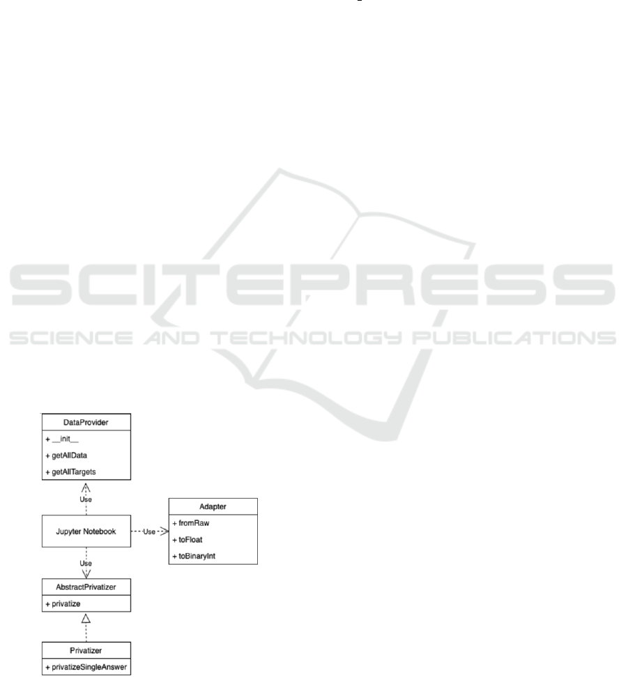
The code was built to be easily extended. You can
plug in a new dataset or your own DP Mechanism. In
Figure 2, there is an UML diagram with the represen-
tation of the architecture. Each Jupyter Notebook has
basically 3 dependencies: DataProvider, Adapter and
Privatizer. The DataProvider is the dataset, with all
the information needed and available to the analysis.
Adapter is simply a class that adapts the format of the
data from DataProvider to the format of the Priva-
tizer.
Privatizer is the class responsible for implement-
ing the DP Mechanism. All privatizers must inherit
from the AbstractPrivatizer abstract class. The ab-
stract class implements the privatize method, that es-
timates the sensitivity of the data (when it is not pro-
vided) and, for each value, adds the noise. The shape
of the noise is implemented inside privatizeSingleAn-
swer. We then implemented the Laplace Mechanism,
which is available in privatizers/laplacePrivatizer.py.
Figure 2: DP lab architecture.
Tests are really important in any code development,
that’s why there are tests for most of the .py files. The
script that runs all of the tests is the runAllTests.sh.
Every time you change something from the existing
code, make sure all the tests pass.
3.2 Methodology and Results
The dataset for the experiments was named
fetch
covtype. It is a tree-cover type dataset
(the predominant type of tree cover) available inside
scikit-learn, an open source, simple and efficient
set of tools for data analysis. This dataset contains
581,012 samples, with a dimensionality of 54 and 7
possible classes. For the initial investigation, we add
noise to attributes and target (classes).
We implement the analysis of the data for the fol-
lowing classification technique: Decision Tree, Na
¨
ıve
Bayes, MLP and SVM. We use the libraries avail-
able in scikit-learn. Inside the notebooks (one for
each technique), there is a section where we adjust
the size of the training data. We can define an array
with all training data sizes to test, and for each size of
choice, there is a random selection of samples from
the database. All the samples that are not used in the
training are then considered in the testing, in order to
measure the accuracy of the algorithm.
Firstly there is the model training using the raw
data. After that, there are multiple data trainings with
different values for ε in the Laplace Mechanism that
is ε-differentially private. All the values of ε are de-
fined in an array as well. After training the model
with the noisy data for different values of ε, all the
results of accuracy are printed in graphs. Here we
show the results for a fixed size of training data. We
use 1,000 samples for Decision Tree, SVM and MLP
techniques. We use 100 samples for training in Na
¨
ıve
Bayes algorithm, due to limited processing time. The
varying value for this experiment is then the ε value.
For Decision Tree algorithm, results are in Fig-
ure 3. We can observe that the bigger the ε value
(which leans less privacy), the closer the accuracy of
the model is compared to the model trained without
privatized data. It is possible to see the convergence
of values. Besides, for very small values of ε there is
a less consistent accuracy. For Na
¨
ıve Bayes algorithm
presented in Figure 4, the behavior is very similar to
the Decision Tree experiment, with the difference of
a faster convergence of values when decreasing the
privacy level (i.e. increasing of ε value).
According to Figure 5, the SVM experiment
shows the same convergence pattern, but with a
slower convergence compared to the previous experi-
ments and also a more stable response for very small
values of ε. The MLP experiment (presented in Figure
ICEIS 2021 - 23rd International Conference on Enterprise Information Systems
880
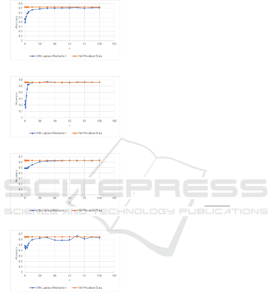
Figure 3: Accuracy of Decision Tree algorithm.
Figure 4: Accuracy of Na
¨
ıve Bayes algorithm.
Figure 5: Accuracy of SVM algorithm.
Figure 6: Accuracy of MLP algorithm.
6) is the one with less stable results, and also the one
with the biggest difference in accuracy between the
model with privatized and not privatized input data.
But it is still possible to recognize a convergence pat-
tern, even though it is not as uniform as the previous
experiments. In all experiments there was a common
pattern, as expected: less privacy means closer results
between using privatized and non-privatized data.
3.3 Analysis
We already know that privacy in differentially private
algorithms can be measured by the ε value. But what
values of ε in a ε-differentially private mechanism are
good and really preserve the privacy? How to under-
stand the impact of the ε value? Thinking about this
question, we propose a more intuitive way of under-
standing such value, and we called it D Coefficient. D
Coefficient is based on the Coin Mechanism (Warner,
1965), described in Section 2.1.
The Coin Mechanism considers that there are two
possible responses (for instance, Yes or No) of a per-
son for a question. When registering someone’s an-
swer, a first coin is tossed. If the result is Heads, it
is registered the answer the person gave. On the other
hand, if the result is Tails, the coin is tossed again. Be-
ing the second result Heads, it is registered Yes; being
Tails, the response is then considered as No.
For defining D Coefficient, the modification we
made was in the first coin toss of the Coin Mech-
anism. Instead of getting a 50% chance of getting
heads, we decided we would get a D chance of get-
ting heads. In other words, the probability of saving
the true answer ’A’ (and not generating it artificially)
will be D, as illustrated in Figure 7. D probability is
itself the D Coefficient that can be calculated, based
on the ε value we want to achieve, as:
D(ε) =
exp(ε) − 1
exp(ε) + 1
D Coefficient represents the chance of saving the orig-
inal answer, if a Coin Mechanism with the same pri-
vacy level was used. The entire demonstration of this
formula is out of the scope of this paper. Considering
the data from the four classification algorithms previ-
ously presented, we calculated the value of ε*. We
define ε* as the minimal ε that gives us less than 10%
difference between accuracy without privacy and ac-
curacy with privacy. We chose 10% in order to have
low interference of DP in the analysis, which means
that it would be possible to achieve similar findings
using privatized data.
We then calculate D(ε*). For N
¨
aive Bayes, we
found ε* = 4 and D(ε*) = 0.964028. For the other
classification algorithms, we found ε* = 10 and D(ε*)
= 0.999909. We observed that D value was very close
to 1, which is not a good finding. It means that if we
use ε* as the privacy level in the Coin Mechanism, the
chances of the first coin toss outputting Heads would
be incredibly high (over 95% for all the experiments).
So, the data would be not privatized as expected, since
the majority of records would keep the original data.
Exploring Differential Privacy in Practice
881
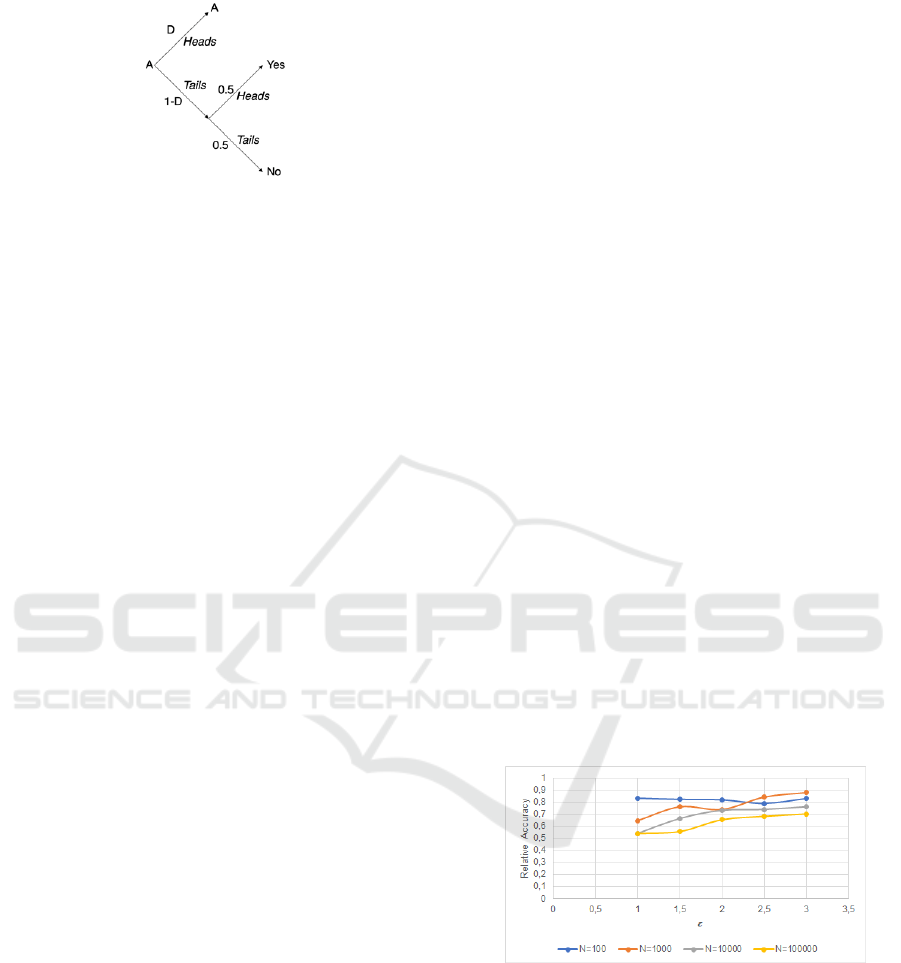
Figure 7: Coin mechanism diagram with variable coin prob-
ability D in the first toss.
3.4 More Investigations
One of the parameters that was kept constant in the
last experiment was the training data size, i.e. how
many samples we used to train each model. For each
classification, we did not vary the amount of data used
in the training. Now we investigate if more samples
can give as better accuracy when dealing with DP.
Given the results from D coefficient, here we use val-
ues of ε between 1 and 3 (which are values of privacy
of our interest).
We calculate the relative accuracy for different
training data sizes and different ε values. The relative
accuracy is defined by dividing the accuracy of the al-
gorithm that used privatized data by the accuracy of
the algorithm trained with the raw data. This mea-
surement (relative accuracy) was chosen because we
expect the accuracy of the model with no privatized
data to increase as the training data increases in size.
We ran each experiment five times, and the output is
the average of found values.
Figure 8 shows the relative accuracy for the Deci-
sion Tree algorithm, where N represents the number
of samples in the training dataset. We found no im-
provement in the relative accuracy when increasing
the size of the input data. Actually, for the biggest
input size we got the worst results. The Na
¨
ıve Bayes
algorithm, presented in Figure 9, does not follow the
behavior of the Decision Tree when comparing the
relative accuracy. Here we have a more optimistic re-
sult: the best results are the ones with the biggest in-
put sizes. For the MLP algorithm, shown in Figure 10,
we observed an unexpected behavior, where it is pos-
sible to highlight that the worst result came from the
biggest training dataset. Results of SVM algorithm,
presented in Figure 11, also indicate that the bigger
the input size, the worse is the relative accuracy.
In the chosen database, there are seven possible
classification of the predominant type of tree cover
(integer value from 1 to 7). The noise, on the other
hand, is a real number drawn from a random vari-
able (driven from the Laplace mechanism). In the first
experiment, we added noise (related to ε value) also
to the classification number, and then rounded the re-
sulting number to match one of the possible classifi-
cations. Here we investigate the application of noise
only to the attributes and not to the target (classes).
We then compare three values here: accuracy with
no privatization, accuracy with full privatization and
accuracy with ’semi- privatization’ (no noise in the
target). We keep the training dataset size fixed. We
made five rounds to get each value, and the results
present the average value of all these rounds. For the
Decision Tree algorithm presented in Figure 12 (for
N = 10,000), both lines where data is somehow pri-
vatized are close to each other, suggesting that keep-
ing the original values for the target data does not add
utility to the privatized data. A similar, but even more
optimistic patter, emerges in the Na
¨
ıve Bayes exper-
iment, as shown in Figure 13 shows (for N = 100).
The fully privatized data gets better results compared
to the semi-privatized in most of points in the chart.
The MLP algorithm, shown in Figure 14 (for N =
10,000) has points with better results with the fully
privatized data compared to the semi-privatized. For
the SVM algorithm presented in Figure 15 (for N
= 1,000), the results are very close to the Decision
Trees, with not much gain in utility by removing the
noise from the target. Similar results were found for
the analyzed classification algorithms, which means
that removing the noise from the target data does not
translate to a gain in overall data utility. It is important
to point out that not privatizing the target data does de-
crease the level of privacy of the data. It makes easier,
for instance, to implement a linkage attack.
Figure 8: Relative accuracy for Decision Tree algorithm by
varying dataset size.
4 CONCLUSIONS
We studied how the theory of Differential Privacy re-
lates to its application, by analysing the impact of DP
mechanisms in the utility of the data for different data
analysis algorithms. In fact we used four classifica-
tion techniques: Decision Tree, N
¨
aive Bayes, SVM
and MLP. By utility we mean the possibility of ex-
ICEIS 2021 - 23rd International Conference on Enterprise Information Systems
882
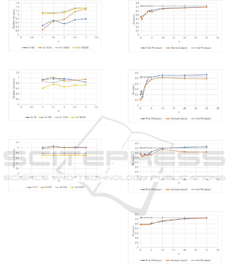
Figure 9: Relative accuracy for N
¨
aive Bayes algorithm by
varying dataset size.
Figure 10: Relative accuracy for MLP algorithm by varying
dataset size.
Figure 11: Relative accuracy for SVM algorithm by varying
dataset size.
tracting good results when using privatized data in-
stead of non-privatized data. In other words, we were
interest to know if the classification techniques could
keep their accuracy in the presence of data privatized
by a DP mechanism.
The path to understand all of these impacts in-
cluded the development of a Differential Privacy Lab.
We projected it with extensibility in mind. Every part
is modular and can be easily replaced. With that de-
cision, we aimed to make a product that was elastic
enough to fit into the workflow of anyone starting to
develop a Differential Privacy solution. We proved
the capabilities of this lab with the experiments we
ran on it, and with all the conclusions we got using
this tool.
During the analysis of the experiment results,
while thinking about the level of privacy, the D Co-
efficient emerged as a more intuitive way of under-
standing the level of privacy of a DP mechanism. We
Figure 12: Accuracy of Decision Tree algorithm consider-
ing distinct application of noise.
Figure 13: Accuracy of N
¨
aive Bayes algorithm considering
distinct application of noise.
Figure 14: Accuracy of MLP algorithm considering distinct
application of noise.
Figure 15: Accuracy of SVM algorithm considering distinct
application of noise.
found that small amounts of noise can lead to a big
drop in utility. It leads to a concern regarding data
privatization, which is that, even with the application
of DP Mechanisms, we cannot say the data is being
properly privatized and maintaining its utility.
Besides, we found that increasing the number of
Exploring Differential Privacy in Practice
883

samples in the training dataset does not always im-
prove accuracy. While removing the noise from the
target data, we observed that there were no significant
gain in utility. In fact, privacy is a little damaged when
data is not fully privatized. Therefore, we encourage
adding noise even to the target data.Of course, more
experiments need to be conducted to confirm our ini-
tial findings.
We believe that the presented experiments as well
the developed lab is a sound basis for understanding
DP and applying it in practice. As future work, we in-
tend to design new experiments considering different
datasets. There can be studied the impact of the pri-
vatization in techniques other than classification ones.
It is also possible to make other types of exploration,
such as combining different DP mechanisms for dis-
tinct parts of the data.
REFERENCES
Abadi, M., Chu, A., Goodfellow, I., McMahan, H. B.,
Mironov, I., Talwar, K., and Zhang, L. (2016). Deep
learning with differential privacy. In ACM SIGSAC
Conference on Computer and Communications Secu-
rity.
Apple (2017a). Learning with privacy at scale. [Online;
accessed 05-Oct-2019].
Apple (2017b). An on-device deep neural network for face
detection. [Online; accessed 11-June-2019].
Buffered.com (2017). The biggest privacy & security scan-
dals of 2017. [Online; accessed 11-June-2019].
Dwork, C. (2006). Differential privacy. In International
Colloquium on Automata, Languages, and Program-
ming (ICALP).
Dwork, C., McSherryKobbi, F., and Smith, N. (2006). Cal-
ibrating noise to sensitivity in private data analysis. In
Theory of Cryptography Conference (TCC).
Dwork, C. and Roth, A. (2014). The algorithmic founda-
tions of differential privacy. Foundations and Trends
in Theoretical Computer Science, 9(3-4):211–407.
Dwork, C. and Rothblum, G. N. (2016). Concentrated dif-
ferential privacy.
Foulds, J., Geumlek, J., Welling, M., and Chaudhuri,
K. (2016). On the theory and practice of privacy-
preserving bayesian data analysis. In Thirty-Second
Conference on Uncertainty in Artificial Intelligence
(UAI).
GDPR (2018). General data protection regulation (gdpr).
Technical report, Official Journal of the European
Union. [Online; accessed 11-June-2019].
Granville, K. (2018). Facebook and cambridge analytica:
What you need to know as fallout widens. [Online;
accessed 11-June-2019].
Havir, D. (2017). A comparison of the approaches to cus-
tomer experience analysis. Economics and Business
Journal, 31(1):82–93.
Jain, P. and Thakurta, A. (2014). (near) dimension indepen-
dent risk bounds for differentially private learning. In
31st International Conference on International Con-
ference on Machine Learning (ICML).
McSherry, F. and Talwar, K. (2007). Mechanism design via
differential privacy. In 48th Annual IEEE Symposium
on Foundations of Computer Science (FOCS).
Minami, K., Arai, H., Sato, I., and Nakagawa, H. (2016).
Differential privacy without sensitivity. In 30th Inter-
national Conference on Neural Information Process-
ing Systems (NIPS).
Mironov, I. (2017). Renyi differential privacy. In IEEE 30th
Computer Security Foundations Symposium (CSF).
Smith, B. and Linden, G. (2017). Two decades of recom-
mender systems at amazon.com. IEEE Internet Com-
puting, 21(3):12–18.
Warner, S. L. (1965). Randomized response: A survey tech-
nique for eliminating evasive answer bias. Journal of
the American Statistical Association, 60(309):63–39.
Winkler, R. (2017). Cybersecurity startup tanium exposed
california hospital’s network in demos without per-
mission. [Online; accessed 11-June-2019].
World, D. I. (2018). How much data is generated per
minute? the answer will blow your mind away. [On-
line; accessed 11-June-2019].
ICEIS 2021 - 23rd International Conference on Enterprise Information Systems
884
