
A Low-Complexity Algorithm for NB-IoT Networks
Salem Alemaishat
School of Computing and Informatics, Al-Hussein Technical University KHBP, Amman 11855, Jordan
Keywords: NB-IoT, 5G, 3GPP, Algorithms.
Abstract: The NB-IoT is a brand-new narrowband IoT technology based on cellular networks. It is an international
standard defined by the 3GPP organization. It can be widely deployed worldwide. It focuses on low-power
wide area networks and operates based on licensed spectrum. It can be directly deployed in The LTE network
has low deployment costs and smooth upgrade capabilities. One of the most influencing factor in NB-IoT
networks is time delay, which affects the system performance. Therefore, this paper proposes an efficient
algorithm to estimate such factor based on the idea of ICI cancellation method to gradually mitigate the
interference between signals in each cell. The proposed algorithm deploys time-frequency cross-correlation
overlapping in each iteration based on the conventional correlation method to further enhance the time delay
estimation accuracy. Furthermore, based on the noise threshold, a first arrival path algorithm is proposed to
eradicate the multipath fading. Simulation results show that the proposed algorithm can effectively improve
the time delay as compared with existing algorithms.
1 INTRODUCTION
The Narrowband Internet of Things (NB-IoT)
proposed in the 3GPP R14 standard supports the
following base station settings:
Position method: Global Assisted Positioning
Satellite System (A-GNSS), E-CID (E-UTRAN cell
identifier), downlink positioning method based on
Observed Time Difference of Arrival (OTDOA) or
uplink based on Observed Time Difference of Arrival
(UTDOA) Positioning method Staniec (2020).
Taking comprehensive consideration of terminal
complexity, network capacity, cost and resources, and
positioning scenarios, if the OTDOA positioning
method is adaptively improved, it can make it more
universal than other positioning methods and more
suitable for a large number of NB-IoT nodes The
positioning cost requirements. The positioning
method based on OTDOA mainly measures the time
delay estimation (TDE) value of 3 or more cell
positioning reference signals (PRS) reaching the
positioning terminal, and estimates the position of the
terminal when the position of each base station is
known. Delay estimation is a very important factor in
the positioning of NB-IoT based on OTDOA.
The representative of the classic delay estimation
algorithm is the cross-correlation method (Knapp,
2003), which estimates the signal delay by searching
for the correlation peak between the local PRS signal
and the received signal. Power consumption and low
cost are required, but the accuracy of time delay
estimation is seriously affected by the system
sampling rate, which makes it not suitable for
accurate positioning of NB-IoT devices with a low
sampling rate (i.e. 1.92 MHz). The super-resolution
delay estimation algorithm (Deng, 2020; Saraereh,
2020; Gu, 2017) increases the cost of IoT devices due
to complexity issues and affects its power
consumption. In addition, due to the building and
terrain, the structure of the mobile communication
channel is complicated. The PRS signals sent by
different cells reach the positioning terminal through
multiple paths. In this process, the signals between
the cells interfere with each other, and the signals in
the cells are also due to multipath effects. Will be
affected by non-line-of-sight (NLOS) (Shahjehan,
2020), these factors will cause delay estimation errors
and even obvious errors. Many scholars have
proposed some algorithms to suppress the influence
of NLOS and eliminate inter-cell interference (Lee,
2018; Khan, 2018; Hu, 2017), but most of these
algorithms are more complex, such as the continuous
interference elimination based on expectation
maximization (EM-SIC) Algorithm, which will cause
relatively large system overhead. Although some
existing time delay estimation algorithms based on
cross-correlation (Ye, 2016; Sun, 2016; Jameel,
2019) have improved accuracy, they fail to
Alemaishat, S.
A Low-Complexity Algorithm for NB-IoT Networks.
DOI: 10.5220/0010439802050214
In Proceedings of the 6th International Conference on Internet of Things, Big Data and Security (IoTBDS 2021), pages 205-214
ISBN: 978-989-758-504-3
Copyright
c
2021 by SCITEPRESS – Science and Technology Publications, Lda. All rights reserved
205

systematically consider inter-cell signal interference
and NLOS effects.
In response to the above problems and combined
with the 3GPP R14 standard, this paper proposes a
delay estimation algorithm based on inter-cell
interference cancellation. On the one hand, the
algorithm separates the delay estimation of the
serving base station and neighboring base stations,
first reconstructs the received signal from the serving
base station, and on this basis, eliminates the strong
interference of the serving base station signal, and
then uses the iterative continuous interference
cancellation algorithm to gradually remove the
received signal. The mutual interference between
signals from neighboring base stations. On the other
hand, in order to break through the limitation of low
sampling rate, this algorithm proposes a time-
frequency cross-correlation overlapping delay
estimation algorithm (F&T_TDE) on the basis of
traditional correlation algorithms, which mainly
includes the following two stages:
In the first stage, multiple OFDM symbols are
combined to obtain a preliminary time delay
estimation value using related algorithms, and the
first path search algorithm based on noise threshold is
used to suppress the impact of multipath effects.
In the second stage, a part of the received signal
is selected for interpolation processing to obtain an
accurate time delay estimate. In addition, considering
the extreme conditions in the project implementation,
there may be less than 3 locating base stations, which
makes the algorithm proposed in this paper unable to
estimate the location of the terminal equipment. An
auxiliary positioning algorithm to deal with such
situations. Common non-base station positioning
algorithms include GPS positioning, anchor node
positioning, fingerprint positioning and other
methods. Taking into account the low power
consumption, low-cost characteristics of NB-IoT, and
the total cost of positioning, the introduction of
anchor node positioning is more practical. Finally,
several commonly used performance indicators of the
time delay estimation algorithm and the performance
of auxiliary positioning are analyzed through
simulation, and the feasibility of the proposed
algorithm is verified.
2 SYSTEM MODEL
According to the 3GPP protocol (Staniec (2020)), the
PRS signal should be transmitted in 𝑁
consecutive
positioning subframes, where 𝑁
is configured by a
higher-level protocol, referring to the principle of
PRS generation in the 3GPP protocol, it can be
obtained that when 𝑙𝑁≤𝑛<(𝑙+1)𝑁, the time
domain PRS signal is
𝑠
,
(𝑛)=
1
√
𝑁
𝑆
,
(𝑘)𝑒
(1)
Among them, 𝑝=0 indicates that the signal
comes from the serving base station, 𝑝=
1,2,… ,𝑃 −1 𝑃 indicates the number of base
stations involved in positioning) indicates that the
signal comes from different neighboring base
stations. A wireless subframe has 2 time slots, and a
time slot includes 7 OFDM symbols, then the number
of OFDM symbols in a positioning subframe is 𝐿=
14 , 𝑙∈
0,1,2,…,𝐿
. 𝑁 represents the length of
inverse fast Fourier transform (IFFT); 𝑆
,
(𝑘) is the
frequency domain PRS signal corresponding to the l
OFDM symbol of the 𝑝 base station after resource
mapping. After adding a guard interval of 𝑁
in
length, the corresponding PRS signal sent in the time
domain is expressed as, 𝑆
,
(𝑛) . The transmitted
signal reaches the receiving end through 𝑀 paths, and
the received signal in the time domain of path 𝑚 for
the 𝑙th OFDM symbol corresponding to the NB-IoT
device terminal is
𝑦
,
(
𝑛
)
=𝛽
ℎ
(
𝑛
)
𝑠
,
(𝑛 −𝜏
,
)
(2)
Where, 𝑙𝑁
≤𝑛<(𝑙+1)𝑁
, 𝑁
=𝑁+𝑁
;
ℎ
(
𝑛
)
=ℎ
𝑒
, 𝛽
and ℎ
are the amplitude
attenuation factor and initial amplitude of the 𝑚th
branch of the signal sent by the 𝑝th cell, respectively;
𝜏
,
is the delay number of the branch path. Adding
the noise 𝑤
(
𝑛
)
in the channel, the final total signal
received at the equipment terminal is
𝑦
(
𝑛
)
=
∑∑∑
𝑦
,
(
𝑛
)
+
𝑤
(
𝑛
)
(3)
Let 𝑟
,
(
𝑛
)
denote the signal, 𝑠
,
(
𝑛
)
and the
cross-correlation function of 𝑦
(
𝑛
)
, as shown in
equation (4).
𝑟
,
(
𝑛
)
=𝐸𝑠
,
(
𝑛
)
𝑦
(
𝑛
)
=𝑅
𝑛 − 𝜏
,
(4)
From the Hermit property of the autocorrelation
function and the characteristic that the origin reaches
the maximum value (Jabeen (2019)), that is
𝑅
(
𝜏
)
=𝑅
∗
(
−𝜏
)
|
𝑅
(
𝜏
)|
≤𝑅
(
0
)
(5)
It can be seen from equation (5) that when 𝑛=
𝜏
,
, then 𝑟
,
(
𝑛
)
takes the maximum value, and the
initial delay number 𝜏
,
is subtracted, and finally
IoTBDS 2021 - 6th International Conference on Internet of Things, Big Data and Security
206

the delay estimate is obtained, 𝑡
̂
,
is shown in
equation (6).
𝑡
̂
,
=𝜏
,
−𝜏
,
𝑇
(6)
Among them, 𝑇
represents the time interval of
sampling points.
3 PROPOSED ALGORITHM
From equations (2) to (5), it can be seen that in the
process of delay estimation, the following three
problems are mainly faced: 1) Interference from
signals sent by other base stations; 2) The influence
of NLOS caused by its own multipath effect; 3) NB-
IoT has a low sampling rate, which seriously affects
the precision of traditional correlation delay
estimation algorithms. In response to the above
problems, the Inter-Cell Interference Elimination
Algorithm (I_SIC) is introduced to eliminate the
mutual interference between signals in multiple
iterations. In each iteration, the F&T_TDE algorithm
is used to estimate the delay estimation value, and the
optimal delay is selected at the end of the iteration.
The estimated value is substituted into the positioning
solution algorithm to estimate the position
coordinates of the terminal. In addition to the above
three problems, in the real environment, there may be
a situation where the number of positioning base
stations is less than three and the algorithm may fail.
Therefore, a supplementary algorithm is given in
section 3.4 to deal with this special situation. When
the number of base stations is greater than 3, the main
body delay estimation algorithm is used, and the Chan
algorithm (Chan, 1994) is used for positioning
solution; otherwise, the auxiliary positioning
algorithm is used. The overall idea of this article and
the main body of the NB-IoT delay estimation
algorithm architecture based on inter-cell interference
cancellation is shown in Figure 1.
End
Number
of BS
𝑃>3
Estimate time delay
Chan location solution
algorithm
Start
Anchor node assisted
positioning
F&T_TDE
I_SIC
F&T_TDE
F&T_TDE
⋮
Figure 1: Proposed algorithm flowchart.
3.1 Algorithm Flow
The cell reference signal (CRS) is continuously sent,
and the CRS signal sent by the serving base station is
less interfered by other base station signals.
Therefore, the CRS signal is used to estimate the
channel of the serving base station and the user
terminal before receiving the PRS signal (Weng,
2010). The method for processing the estimated time
delay from each base station to the terminal is as
follows: First, use the CRS signal to estimate the
channel state between the serving base station and the
terminal. Second, at the receiving end, receive the
PRS signals from each base station, and use the
existing channel state between the serving base
station and the terminal to reconstruct the PRS signal
of the serving cell at the receiving end, and use the
F&T_TDE algorithm to estimate the time delay of the
serving base station; Finally, the reconstructed PRS
signal from the serving base station is subtracted from
the total received PRS signal to eliminate its influence
on the delay estimation of the neighboring base
station. On this basis, a continuous iterative
interference cancellation algorithm is used to
gradually eliminate the signal between neighboring
cells. At the same time, the F&T_TDE algorithm is
used to estimate the delay of the serving base station.
Algorithm 1: Proposed algorithm for delay estimation.
Initialization: 𝑦
,
(𝑛)←𝑦(𝑛)
1: if 𝑝=0
2: 𝑁
←1, 𝑞←1
3: Determine 𝑡
̂
,
4: 𝑡
←𝑡
̂
,
5: Determine 𝑦
,
(𝑛)
6: Obtain 𝑦
,
(
𝑛
)
←𝑦
,
(
𝑛
)
−𝑦
,
(𝑛)
7: Else
8: for 𝑞=1 to 𝑁
9: for 𝑝=1 to 𝑃−1
10: Determine 𝑡
̂
,
11: Obtain 𝑦
,
(𝑛)
12: if 𝑝<𝑃−1
13: Obtain 𝑦
,
(
𝑛
)
14: Else
15: 𝑦
,!
(
𝑛
)
←𝑦
,
(
𝑛
)
−𝑦
,
(𝑛)
16: end if
17: 𝑝=𝑝+1
18: end for
19: 𝑞=𝑞+1
20: end for
21: 𝑡
=min𝑡
̂
,
22: end if
A Low-Complexity Algorithm for NB-IoT Networks
207

After multiple iterations of interference elimination,
the best delay estimate is selected. The pseudo-code
of the main body delay estimation algorithm is shown
in Algorithm 1, where 𝑦(𝑛) represents the total
received signal of the device terminal; 𝑦
,
(𝑛) and,
𝑡
̂
,
respectively represent the 𝑝th after 𝑞 iterations,
time-domain received signal and time delay
estimation value of the cell; 𝑡
represents the final
time delay estimation value obtained by the 𝑝th cell,
and 𝑁
is the number of interference cancellation
iterations.
3.2 F&T_TDE Algorithm
Inter-cell interference cancellation can only suppress
the interference signals of other cells to a certain
extent, and cannot solve the problem of low sampling
rate of the NB-IoT system. To greatly improve the
accuracy of time delay estimation, it is necessary to
improve the time delay estimation algorithm. In order
to improve the serial interference and avoid error
propagation, before the time delay estimation is
performed, the transmitted PRS signal is first based
on the order of the time delay estimation from each
neighboring base station to the terminal according to
its energy, and then through 2 stages Gradually
improve the accuracy of time delay estimation.
3.2.1 Rough Estimation of Delay Value
First, starting from the time 𝑛
,
(the initial time of
receiving the lth OFDM symbol of the 𝑝 th base
station), sample the time domain signal received in
the 𝑞th iteration, 𝑦
,
(
𝑛
)
, and get 𝑁
. The received
signal at the sampling point, denoted as 𝑦
,
,
(𝑛).
Secondly, using a sampling point as a sliding
window, the received signal starting at 𝑛
,
is
obtained in sequence as described above, 𝑦
,
,
(𝑛),
where, 𝑛
,
=𝑖+𝑙𝑁
, 0≤𝑖<𝑁
. Then, perform
FFT transformation on 𝑦
,
,
(𝑛) to obtain
𝑌
,
,
(
𝑘
)
,𝑌
,
,
(
𝑘
)
,… ,𝑌
,
,
(𝑘) and perform the local
positioning reference signal corresponding to the 𝑙
OFDM symbol of the 𝑝 base station with 𝑌
,
,
(
𝑘
)
frequency-domain correlation operation is performed
to obtain the corresponding OFDM symbol 𝑙
and
delay number 𝑛
,
when the correlation function of
the base station 𝑝 is maximized, as shown in equation
(7).
𝑛
,
,𝑙
=𝑆
,
(
𝑘
)
𝑌
,
,
(
𝑘
)
𝑘 −𝑛
,
∗
,
,
(7)
Among them, when 𝑝=0, 𝑞=1, and 𝑝>0, and
𝑞∈
1,2,…,𝑁
; 𝑁
represents the total number of
iterations of the continuous interference cancellation
algorithm. 𝑛
,
−𝑛
,
, which is the number of delays
in the rough estimate of the 𝑞th iteration. Since noise
and multipath effects will cause NLOS effects, the
time delay value obtained at this time has a large
error, so this paper uses the first path search algorithm
to reduce the error. The specific implementation
process of the algorithm is as follows.
Before the signal arrives, the receiver first collects
the noise signal and converts it into a frequency
domain signal 𝑊
(
𝑘
)
, and correlates it with the local
PRS signal in the frequency domain, repeats Φ times,
and obtains the average value as shown in equation
(8) (mean noise floor).
𝑅
=
∑∑
𝑆
,
(
𝑘
)
𝑊
∗
(
𝑘
)
(8)
Set the noise floor threshold as 𝐿
, the noise
floor threshold and the average value of the noise
floor should satisfy the relationship shown in
equation (9), where the industrial setting κ = 6 dB and
is expressed as
𝜅=10log
𝐿
𝑅
(9)
The frequency domain received signal
corresponding to the OFDM symbol 𝑙
with the
largest peak value obtained by the rough estimation
of the time delay value, 𝑌
,
(
𝑘
)
is correlated with the
local PRS signal in the frequency domain to obtain
the correlation function, 𝑅
,
,
(
𝑘
)
, where 𝑘∈
𝑙
𝑁
,𝑙
+1𝑁
.
𝑅
,
,
(
𝑘
)
=𝑅
(
𝑘
)
+𝑅
(
𝑘
)
(10)
Among them, 𝑅
(
𝑘
)
represents the
correlation function between the useful signal and the
interference signal and the local PRS signal, and
𝑅
(
𝑘
)
represents the correlation function between
the noise and the local PRS signal. In order to
accurately estimate the required cell delay value, it is
necessary to eliminate the influence of the
interference signal, so the noise floor threshold is
introduced to obtain the 𝑅
(
𝑘
)
shown in equation
(11).
IoTBDS 2021 - 6th International Conference on Internet of Things, Big Data and Security
208

𝑅
(
𝑘
)
=
𝑅
,
,
(
𝑘
)
max𝑅
,
,
(
𝑘
)
𝐿
(11)
When the amplitude of the first path signal is
small, the useful signal will be overwhelmed by noise
and interference signals, and it is impossible to
determine the final required delay estimate based on
the first path delay value. Therefore, an amplitude
threshold 𝛼 is set. When the amplitude of the first
arrival path is less than the threshold, a suboptimal
path will be selected, and the instant delay value is
only greater than the path of the first arrival path, thus
the first arrival path search formula can be obtained
as (12) shown.
𝑛
,
= 𝑅
,
,
(
𝑘
)
>𝛼max𝑅
,
,
(
𝑘
)
𝑅
,
,
(
𝑘
)
max𝑅
,
,
(
𝑘
)
𝐿
(12)
Among them, 𝑛
,
is the delay number of the
first path.
3.2.2 Time Delay Fine Estimation Stage
First, let, 𝑣
,
∈𝑛
,
−∆𝜇,𝑛
,
+∆𝜇, the value of
𝑣
,
is
∆
; Secondly, for the time-domain received
signal corresponding to the 𝑙
OFDM symbol,
𝑦
,
𝑣
,
+
∆
interpolates to obtain the signal
𝑦
,
,
, where 𝑖∈
0,1,…,𝑁
−1
, interpolation
function set. The expression is shown in equation
(13).
𝑦
,
,
(𝑖)
=
𝑦
,
(
floor(𝜓)
)
floor
(
𝜓
)
<𝜓<ceil
(
𝜓
)
−0.5
𝑦
,
(
ceil(𝜓)
)
ceil
(
𝜓
)
−0.5<𝜓<ceil
(
𝜓
)
+0.5
(13)
Among them, 𝜓=𝑣
,
+
∆
, floor
(
𝜓
)
represents rounding 𝜓 to the −∞ direction, ceil
(
𝜓
)
represents rounding 𝜓 to the +∞direction, ∆𝜇
represents the selected time-domain interpolation
range, and 𝜔 represents the number of points for time
domain interpolation.
The processed received signal 𝑦
,
,
(𝑖) is
correlated with the local PRS signal corresponding to
the selected base station 𝑝 in the time domain, and the
accurate time delay estimation value from the 𝑝th
base station to the terminal at the 𝑞th iteration is
obtained, 𝑡
̂
,
, as in equations (14) as shown.
𝚤
̂
,
=𝐸𝑆
,
𝑖+ 𝑙
𝑁
𝑦
,
,
(𝑖)
𝑡
̂
,
=𝑛
,
−∆𝜇+
2∆𝜇𝚤
̂
,
𝜔
−𝑙
𝑁
(14)
We use the channel estimation algorithm
described in below section to obtain the channel state
between the base station 𝑝 and the terminal, and
reconstruct the received signal from the base
station,𝑦
,
(
𝑛
)
, and subtract from the received signal,
𝑦
,
(𝑛) is the reconstructed signal obtains equations
(15) and (16).
If 𝑝<𝑃−1, then
𝑦
,
(
𝑛
)
=𝑦
,
(
𝑛
)
−𝑦
,
(
𝑛
)
(15)
If 𝑝=𝑃−1 and 𝑞≤𝑁
, then
𝑦
,
(
𝑛
)
=𝑦
,
(
𝑛
)
−𝑦
,
(
𝑛
)
(16)
3.2.3 Channel Estimation
In order to reduce the computational complexity of
the algorithm, this paper uses the least square method
to estimate the channel of the positioning reference
signal from the base station p to the user terminal.
When 𝑝=0, channel estimation is performed on the
CRS signal of the serving base station, and the system
function is obtained as shown in equation (17).
𝑯
,
=𝑺
,
𝒀
(17)
Among them, 𝒀
and 𝑺
,
respectively
represent the CRS signal received by the terminal and
the CRS signal sent by the serving base station.
Perform linear interpolation on this system function
(Bohanuding (2010)) to obtain the channel estimation
of the time-frequency position of the PRS signal, and
perform IFFT transformation on it to obtain ℎ
,
(
𝑖+
𝑙𝑁
)
, where 𝑖=0,1,2,… ,𝑁
−1. The reconstructed
signal from the serving base station is
𝑦
,
(
𝑛
)
=
∑
ℎ
,
(
𝑛
)
𝑆
,
𝑛 − 𝑣
,
(18)
Where, 𝑛∈
𝑙𝑁
,
(
𝑙+1
)
𝑁
.
At this time, 𝑝>0, and the system function is
obtained as shown in equation (19).
ℎ
,
(
𝑖+𝑙𝑁
)
=IFF
𝑌
,
(
𝑘
)
𝑆
,
(
𝑘
)
(19)
According to the system function shown in
equation (19), the received signal from the base
station 𝑝 is reconstructed, and the reconstructed
signal is
𝑦
,
(
𝑛
)
=
∑
ℎ
,
(
𝑛
)
𝑆
,
𝑛 − 𝑣
,
(20)
Where, 𝑛∈
𝑙𝑁
,
(
𝑙+1
)
𝑁
.
A Low-Complexity Algorithm for NB-IoT Networks
209

3.2.4 Anchor Node Location Algorithm
The DV-Hop positioning algorithm is one of the key
technologies for anchor node positioning. It adopts a
distance vector-hop mechanism, does not need to
measure the distance between nodes, and does not
require additional hardware support. It is a distance-
independent (range- free) algorithm. This article
chooses DV-Hop algorithm as the auxiliary
positioning algorithm. For areas with less deployment
of base stations, when the number of base stations is
less than 4 (the position estimation deviation is
relatively large when the number of base stations is
3), the terminal device node broadcasts a positioning
data packet to the anchor node, and the anchor node
records the receiving time of receiving the data packet
Stamp and the ID of the terminal node to be located.
At the same time, the anchor nodes perform time
synchronization through satellite navigation and
obtain terminal device node geographic location data
and store it in the background server to provide
relevant parameters for algorithm processing. Each
anchor node sends a new data packet to the gateway,
and the gateway forwards the new data packet to the
background server, and uses the weighted centroid
algorithm to estimate the position coordinates of the
terminal node (Qiang (2020)). It should be noted that
the anchor node location algorithm, as an auxiliary
part of the algorithm proposed in this article, only
works when the main algorithm fails.
4 SIMULATION RESULTS
This section provides the numerical simulation results
with elaboration. The proposed algorithm is evaluated
from different important aspects.
4.1 Simulation Parameters Settings
During the simulation, due to the synchronous
network mode, the wireless subframes sent by all base
stations are aligned in the time domain. Since the NB-
IoT network is mainly for macroscopic and low-speed
objects, the simulation assumes that the device
terminal. The moving speed is 0 km/s, and other
simulation parameters are set according to the PRS
signal in 3GPP R14 and based on the OTDOA
positioning method (Mwakwata (2019)). The specific
parameter settings are shown in Table 1. The NB-IoT
device terminal nodes (solid nodes) scattered in the
dark gray area are randomly selected, and m anchors
are fixed in a grid in each 500 m × 500 m area node
and configure the GNSS positioning module as a
reference node for positioning. When the number of
base stations involved in positioning is less than 4,
anchor node positioning is enabled. When studying
the influence of distance on time delay estimation, the
equipment terminal in the direction 1 area as shown
in Figure 2(b) is selected. In addition, select the 4 base
stations closest to the terminal as the positioning base
station, where base station 0 (located in the center of
the serving cell) is the serving base station, and base
station 1/2/3 (located in the center of the neighboring
cell 1/2/3) is the neighboring base station.
Table 1: Simulation Parameters.
Parameter Value
Number of BS and NB-IoT
antennas
1
Number of terminal nodes 5000
Number of base stations 4
Base station spacing 1732 m
Moving speed of terminal
equipment
0 km/s
𝑁
1
𝑁
3
CP type Conventional CP
Sampling rate 𝐹
1.92 MHz
∆𝑡 1𝐹
⁄
2∆𝜇 𝜔
⁄
0.01
Path loss
𝐿
=120.9 + 37.6 𝑑
Channel model AWGN
In the simulation, the delay estimation based on
the positioning reference signal mainly uses the
detection probability (PD) of the delay estimate, the
root mean square error (RMSE) of the delay
estimation and the cumulative distribution function
(CDF) of the device terminal positioning error. To
measure the positioning effect, the positioning error
is mainly used to measure the auxiliary positioning
based on anchor nodes.
4.2 Simulation Results Analysis
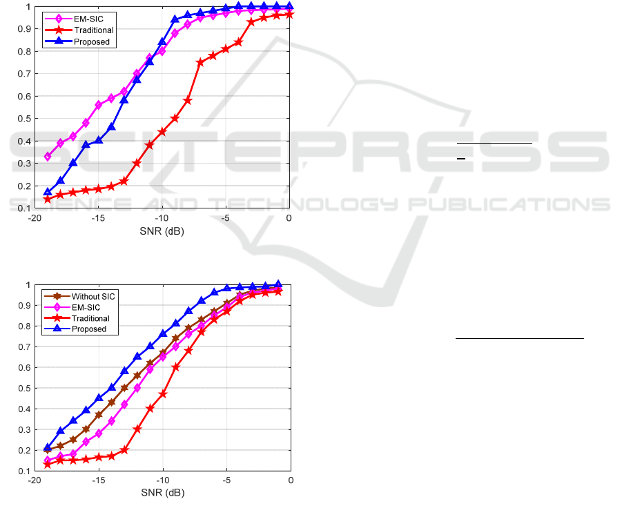
4.2.1 Probability of Detection
In this paper, the detection probability refers to the
probability that the estimated time delay 𝑡
̂
is within a
given threshold 𝑇 in 𝑀 Monte Carlo simulation
IoTBDS 2021 - 6th International Conference on Internet of Things, Big Data and Security
210
experiments. In order to satisfy that users
participating in positioning are located within the
coverage of the serving base station, the threshold
here is 𝑇
=5.78×10
s, the instant delay
error is less than the propagation time of the signal
from two adjacent base stations. In Figure 2, the
number of Monte Carlo simulations is set to 1,000,
and the detection probability PD of the serving cell
and neighboring cell 1 are given as a function of SNR.
As shown in Figure 2(a), when the SNR is greater
than 20 dB, the detection probability shows an
obvious upward trend; when the SNR is less than −12
dB, due to the influence of noise, the detection
probability of the serving cell obtained by the
proposed algorithm and the two comparison
algorithms Very low, and when the signal-to-noise
ratio of the proposed algorithm is too low, the
(a) Comparison of detection probability of serving cell
(b) Comparison of detection probability
of neighboring cell 1
Figure 2: Serving cell and neighboring cell 1 detection
probability varies with SNR.
reconstruction signal error is too large, which
seriously affects the delay estimation, and the
detection probability is lower than the EM-SIC
algorithm; when the SNR is greater than −12 dB, the
detection probability will exceed EM-SIC algorithm;
In addition, compared with the other two algorithms,
the proposed algorithm has a more significant upward
trend in the detection probability curve. Similarly, as
shown in Figure 2(b), for neighboring cell 1 (the
curve trend of neighboring cells 2/3 and 1 is basically
the same), when the SNR is greater than −20 dB, as
the SNR increases, the detection probability becomes
obvious Increasing trend, and the detection
probability of the proposed algorithm is higher than
that of the EM-SIC algorithm and the traditional
algorithm; in order to highlight the effect of inter-cell
interference elimination, Figure 2(b) also shows that
the interference is not added.
In the case of elimination, it can be seen that
adding interference elimination can effectively
improve the detection probability.
4.2.2 RMSE Analysis
The definition of the root mean square error is shown
in equation (21).
𝑅𝑀𝑆𝐸=𝑐
∑(
𝑡
̂
−𝑡
)
(21)
Among them, 𝑐 is the speed of light, and the value
is 3.0×10
8
m/s; 𝑀 is the number of Monte Carlo
simulations and the value is 1 000; 𝑡 is the actual
delay value. In addition, the CRLB lower bound
(CRLB) provides a measure of the error of the delay
estimation. From the literature (Xu (2016)), the
CRLB lower bound of the NB-IoT delay estimation
in the AWGN environment can be expressed as
𝑣𝑎𝑟
𝑡
̂
≥CRLB
𝑡
̂
=
∆
∑∑
,
(
)
(22)
where, ∆𝑓=1 𝑁𝑇
⁄
and 𝜎
is the noise power.
The mean square error of the delay estimation can
be used to measure the accuracy of the delay
estimation.
Figure 3(a) compares the mean square error of the
delay estimation of the serving cell. Since the
proposed algorithm uses the channel estimation of the
cell reference signal to reconstruct the positioning
reference signal of the serving cell, the obtained delay
estimated value is obviously closer to the CRLB
lower bound than the traditional correlation algorithm
and the EM-SIC algorithm.
Detection Probability
Detection Probability
A Low-Complexity Algorithm for NB-IoT Networks
211
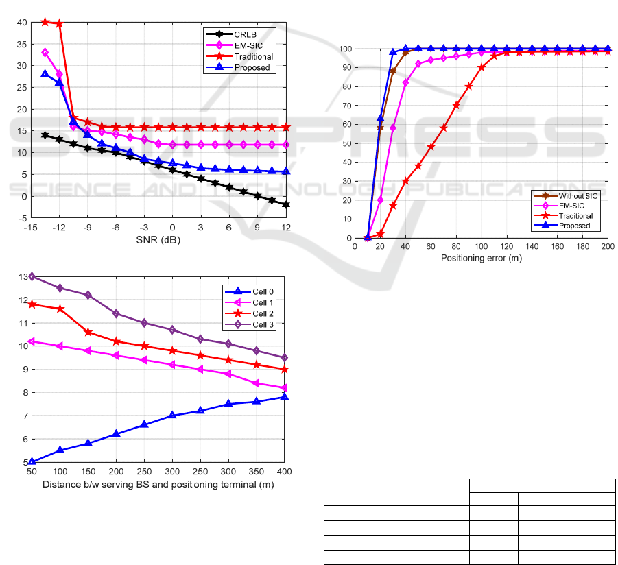
In addition to SNR affecting the delay estimation
result, the distance between the positioning terminal
and the serving base station and neighboring base
stations also affects the delay estimation.
In Figure 3(b), the influence curve of the distance
between the serving base station and the positioning
terminal (along direction 1 in Figure 2(b)) on the
delay estimation is given when SNR=5 dB. It can be
seen that when the distance is small, the mean square
error of the serving cell is relatively small, while
neighboring cells are seriously affected by the serving
cell, and the mean square error of the time delay
estimation is relatively large. As the distance
increases, the mean square error of the serving cell
gradually increases, while the mean square error of
neighboring cells gradually decreases. Therefore, the
importance of inter-cell interference cancellation is
explained from the perspective of the influence of
distance on time delay estimation.
(a)
(b)
Figure 3: Time delay estimation mean square error variation
curve of cell 0/1.
4.2.3 CDF of Positioning Error
When the positioning solution method is determined,
the positioning accuracy of the user terminal is
determined by the accuracy of the delay estimation,
that is, it is jointly determined by multiple delay
estimation values (the delay estimation values from 3
or more base stations to the user terminal). The
simulation in this paper uses the Chan algorithm to
solve the problem, which can reach the CRLB lower
bound when the delay estimation error is small.
Figure 4 shows the comparison of the positioning
error curves of the traditional algorithm, the
algorithm proposed in this paper, and the EM-SIC
algorithm. It can be seen from Figure 4 that the
positioning accuracy of the algorithm in this paper is
significantly higher than the traditional algorithm and
the EM-SIC algorithm. This is because the algorithm
proposed in this paper incorporates interference
cancellation, which improves the positioning
accuracy of the algorithm to a certain extent.
Figure 4: Comparison of positioning error and CDF.
Table 2 shows the positioning errors of different
algorithms for different cumulative errors. As shown
in Table 2, when the cumulative error reaches 50%,
the positioning error of this algorithm can reach 4.27
m, while the traditional algorithm positioning error is
47.56 m, and the EM-SIC algorithm positioning error
is 18.52 m; when the cumulative error reaches 90%,
the gap between the three is even greater.
Table 2: Analysis of positioning error corresponding to
different accumulated errors.
Algorithm CDF
50% 80% 90%
Traditional algorithm 47.56 m 69.46 m 81.18 m
EM-SIC algorithm 18.52 m 28.73 m 39.50 m
Proposed algorithm without IC 5.52 m 8.73 m 10.88 m
Proposed algorithm with IC 4.27 m 6.56 m 8.00 m
RMSE (dBm)
RMSE (dBm)
CDF (%)
IoTBDS 2021 - 6th International Conference on Internet of Things, Big Data and Security
212

4.2.4 Aided Positioning Simulation Analysis
Figure 4 shows the analysis of anchor node
positioning error. It can be seen that the number of
anchor nodes and the communication radius of the
nodes will affect the accuracy of positioning. When
the communication radius of the node is 60 m, the
relationship between the number of anchor nodes and
the positioning error is shown in Figure 3(a). As the
number of anchor nodes increases, the positioning
error gradually decreases, but at the same time,
positioning cost also increases. The communication
radius and the density of anchor nodes also restrict
each other. When the location of the anchor node is
determined, the distance between the nodes is also
determined. The communication radius will affect the
average hop distance of the algorithm, thereby
affecting the positioning accuracy. At this time, the
positioning error of the communication radius first
decreases and then gradually increases. The position
of the turning point is determined by the
communication radius and the density of anchor
nodes. Figure 3(b) shows the relationship between
communication radius and positioning error when
there are 64 anchor nodes. It is worth noting that the
increase in the communication radius is obtained by
increasing the transmission power.
From the above simulation analysis, it can be seen
that to improve the positioning accuracy of the
auxiliary positioning algorithm, the number of anchor
nodes and the communication radius need to be
increased. At this time, the positioning cost will also
increase year-on-year. However, the position
estimation effect of the auxiliary positioning
algorithm is far less than that mentioned in this
article. Delay estimation algorithm, so the auxiliary
positioning algorithm is only used as a backup
solution when the base station is insufficient in real
positioning scenarios.
5 CONCLUSION
This article proposes a delay estimation algorithm
based on inter-cell interference cancellation for the
problems of NB-IoT's cost limitation and low
sampling rate. The algorithm continues the low
complexity advantages of the traditional cross-
correlation algorithm, and uses base stations to
participate in positioning to reduce equipment
overhead, and more satisfies the low power
consumption and low cost characteristics of NB-IoT.
Through simulation analysis, the proposed delay
estimation algorithm can effectively suppress the
influence of inter-cell interference and NLOS. The
delay estimation accuracy is significantly higher than
the comparison algorithm, which is more in line with
today's high-precision location sensing needs. As to
whether there are positioning scenarios with SNR less
than −20dB and whether it is necessary to improve
the TDE accuracy below −20dB, further research is
needed.
ACKNOWLEDGMENT
The authors would like to thank the editors and
reviewers for their review and recommendations.
REFERENCES
K. Staniec, M. Kucharazak, Z. Joskiewics and B.
Chowanski, “Measurement-Based Investigations of the
NB-IoT Uplink Performance at Boundary Propagation
Conditions,” Electronics, vol. 9, no. 11, pp. 1–13, 2020.
C. Knapp and G. Carter, “The Generalized Correlation
Method for Estimation of Time Delay,” IEEE
Transactions on Acoustic Speech & Signal Processing,
vol. 24, no. 4, pp. 320–327, 2003.
Z. Deng, X. Zheng, H. Wang, X. Fu, L. Yin et al., “A Novel
Time Delay Estimation Algorithm for 5G Vehicle
Positioning in Urban Canyon Environments,” Sensors,
vol. 20, no. 18, pp. 1–19, 2020.
O. A. Saraereh, A. Alsaraira, I. Khan and B. J. Choi, “A
Hybrid Energy Harvesting Design for On-Body
Internet-of-Things (IoT) Networks,” Sensors, vol. 20,
no. 2, pp. 1–13, 2020.
Y. Gu and N. A. Goodman, “Information-theoretic
compressive sensing kernel optimization and Bayesian
Cramer-rao bound for time delay estimation,” IEEE
Transactions on Signal Processing, vol. 65, no. 17, pp.
4525–4537, 2017.
W. Shahjehan, S. Bashir, S. L. Mohammed, A. B. Fakhri,
A. D. Isaiah et al., “Efficient Modulation Scheme for
Intermediate Relay-Aided IoT Networks,” Applied
Sciences, vol. 10, no. 6, pp. 1–14, 2020.
B. M. Lee, M. Patil, P. Hunt and I. Khan, “An Easy
Network Onboarding Scheme for Internet of Things
Networks,” IEEE Access, vol. 7, pp. 8763–8772, 2018.
I. Khan and D. Singh, “Energy-balance node-selection
algorithm for heterogeneous wireless sensor networks,”
ETRI Journal, vol. 40, no. 5, pp. 604–612, 2018.
S. Hu, A. Berg, X. Li and F. Rusek, “Improving the
Performance of TDOA Based Positioning in NB-IoT
Systems,” IEEE Global Communications Conference
(GLOBECOM), Singapore, pp. 1–7, 2017.
D. Ye, J. Y. Lu, X. J. Zhu and H. Lin, “Generalized Cross
Correlation Time Delay Estimation Based on Improved
Wavelet Threshold Functionn,” IEEE 6
th
International
Conference on Intrumentation & Measurement,
A Low-Complexity Algorithm for NB-IoT Networks
213

Computer, Communication and Control (IMCCC),
Harbin, China, pp. 629–633, 2016.
H. M. Sun, R. S. Jia, Q. Q. Du et al., “Cross-correlation
Analysis and Time Delay Estimation of a Homologous
Micro-Seismic Signal Based on the Hilbert-Huang
Transform,” Computers & Geosciences, vol. 91, no. C,
pp. 98–104, 2016.
F. Jameel, T. Ristaniemi, I. Khan and B. M. Lee,
“Simultaneous Harvest-and-Transmit Ambient
Backscatter Communications Under Rayleigh Fading,”
EURASIP Journal on Wireless Communications and
Networking, vol. 166, pp. 1–9, 2019.
T. Jabeen, Z. Ali, W. U. Khan, F. Jameel, I. Khan et al.,
“Joint Power Allocation and Link Selection for Multi-
Carrier Buffer Aided Relay Network,” Electronics, vol.
8, no. 6, pp. 1–13, 2019.
Y. T. Chan and K. C. Ho, “A Simple and Efficient
Estimator for Hyperbolic Location,” IEEE
Transactions on Signal Processing, vol. 42, no. 8, pp.
1905–1915, 1994.
G. Weng, C. Yin and T. Luo, “Channel Estimation for the
Downlink of 3GPP-LTE systems,” IEEE International
Conference on Network Infrastructure and Digital
Contents, Beijing, China, pp. 1042–1046, 2010.
S. Bohanuding, M. Ismail and H. Hussai, “Simulation
Model and Location Accuracy for Observed Time
Difference of Arrival (OTDOA) Positioning Technique
in Third Generation System,” IEEE Student Conference
on Research and Development – Engineering:
Innovation and Beyond, Putrajaya, Malaysia, pp. 63–
65, 2010.
L. Qiang, H. Xia, X. Yuhang and Z. Dan, “Improved DV-
Hop Based on Dynamic Parameters Differential
Evolution Localization Algorithm,” IEEE 8
th
International Conference on Information,
Communication and Networks (ICICN), Xi’an, China,
pp. 129–134, 2020.
C. B. Mwakwata, H. Malik, M. M. Alam, Y. L. Moullec, S.
Parand et al., “Narrowband Internet of Things (NB-
IoT): From Physical (PHY) and Media Access Control
(MAC) Layers Perspective,” Sensors, vol. 19, no. 11,
pp. 1–34, 2019.
W. Xu, M. Huang, C. Zhu, et al., “Maximum Likelihood
TOA and OTDOA estimation with first arriving path
detection for 3GPP LTE system,” Transactions on
Telecommunications Technologies, vol. 27, no. 3, pp.
339–356, 2016.
IoTBDS 2021 - 6th International Conference on Internet of Things, Big Data and Security
214
