CC-separation Measure Applied in Business Group Decision Making

Jonata C. Wieczynski

1 a

, Giancarlo Lucca

2,3 b

, Eduardo N. Borges

2 c

, Grac¸aliz P. Dimuro

2,5 d

Rodolfo Lourenzutti

4 e

and Humberto Bustince

5 f

Programa de P

os-Graduac¸

ao em Computac¸

ao, Universidade Federal do Rio Grande, Av. It

alia Km 8, Rio Grande, Brazil

Programa de P

os-Graduac¸

ao em Modelagem Computacional, Universidade Federal do Rio Grande, Rio Grande, Brazil

Centro de Ci

encias Computacionais, Universidade Federal do Rio Grande, Rio Grande, Brazil

Department of Statistics, University of British Columbia, Vancouver, Canada

Departamento de Estad

ıstica, Inform

atica y Matem

aticas, Universidad Publica de Navarra, Pamplona, Spain

Keywords:

Decision Making, TOPSIS, GMC-RTOPSIS, Generalized Choquet Integral, CC-integrals.

Abstract:

In business, one of the most important management functions is decision making. The Group Modular Cho-

quet Random TOPSIS (GMC-RTOPSIS) is a Multi-Criteria Decision Making (MCDM) method that can work

with multiple heterogeneous data types. This method uses the Choquet integral to deal with the interaction be-

tween different criteria. The Choquet integral has been generalized and applied in various ﬁelds of study, such

as imaging processing, brain-computer interface, and classiﬁcation problems. By generalizing the so-called

extended Choquet integral by copulas, the concept of CC-integrals has been introduced, presenting satisfactory

results when used to aggregate the information in Fuzzy Rule-Based Classiﬁcation Systems. Taking this into

consideration, in this paper, we applied 11 different CC-integrals in the GMC-RTOPSIS. The results demon-

strated that this approach has the advantage of allowing more ﬂexibility and certainty in the choosing process

by giving a higher separation between the ﬁrst and second-ranked alternatives.

1 INTRODUCTION

Business managers rely on the right decisions to keep

their business competitive. Many times a decision

has to be made by multiple analysts and considering

various criteria. This is a time consuming and ex-

pensive task. Although, most of the time, it can be

solved by an algorithm or mathematical model, like

route, supplier chain, and location problems (Deveci

et al., 2017; Alazzawi and

Zak, 2020; Shyur and Shih,

2006), releasing the pressure of the decision from the

managers, and allow them to work on other processes

of the company/industry.

The Technique for Order of Preference by Simi-

larity to Ideal Solution (TOPSIS) (Huang and Yoon,

1981) is one of the multi-criteria decision making

(MCDM) methods that ranks the best possible solu-

https://orcid.org/0000-0002-8293-0126

https://orcid.org/0000-0002-3776-0260

https://orcid.org/0000-0003-1595-7676

https://orcid.org/0000-0001-6986-9888

https://orcid.org/0000-0003-2434-4302

https://orcid.org/0000-0002-1279-6195

tion among a set of alternatives. This approach is

based on pre-deﬁned criteria, using the alternative’s

distance to the best and worst possible solutions for

the problems, Positive and Negative Ideal Solutions

(PIS and NIS), respectively.

In 2017, the Group Modular Choquet Random

TOPSIS (GMC-RTOPSIS) (Lourenzutti et al., 2017)

was introduced. The method generalized the orig-

inal TOPSIS allowing it to deal with multiple and

heterogeneous data types. The approach models the

interaction among the criteria by using the discrete

Choquet integral (Choquet, 1954). The Choquet inte-

gral allows a function to be integrated by using non-

additive fuzzy measures (Choquet, 1954; Candeloro

et al., 2019), which means that it can consider the in-

teraction among the elements that are being integrated

(Murofushi and Sugeno, 1989; Dimuro et al., 2020).

The GMC-RTOPSIS learns the fuzzy measure associ-

ated with the criteria with a Particle Swarm Optimiza-

tion (PSO) algorithm (Wang et al., 2011) .

The C

-integrals (Lucca et al., 2016) is a general-

ization of the Choquet integral that replaces the prod-

uct operation by triangular norm (t-norm) functions

(Klement et al., 2011). The C

-integrals are a family

452

Wieczynski, J., Lucca, G., Borges, E., Dimuro, G., Lourenzutti, R. and Bustince, H.

CC-separation Measure Applied in Business Group Decision Making.

DOI: 10.5220/0010439304520462

In Proceedings of the 23rd International Conference on Enterprise Information Systems (ICEIS 2021) - Volume 1, pages 452-462

ISBN: 978-989-758-509-8

of integrals that are pre-aggregation functions (Lucca

et al., 2016). Additionally, C

-integrals are averaging

functions, i.e., the result is always between the mini-

mum and maximum of the input.

The T-separation measure (Wieczynski et al.,

2020) was introduced and applied in the GMC-

RTOPSIS instead of the Choquet integral. In

this study, the authors considered ﬁve different T-

separation measures to tackle Case Study 2 from

(Lourenzutti et al., 2017). The problem consists of

choosing a new supplier for a company by asking var-

ious decision-makers to give their opinions with dif-

ferent criteria. The problem is posed with a variety

of data types, such as probability distributions, fuzzy

numbers, and interval numbers. The paper also pro-

posed to use the t-norm that better discriminates the

ﬁrst ranked alternative to the second one by calcu-

lating the difference of the rankings. The approach

presented good results when using the Łukasiewicz

t-norm (T

), giving a better separation between the

ranked alternatives than the standard Choquet inte-

gral.

After introducing the C

-integrals, Lucca et al.

have proposed the CC-integrals (Lucca et al., 2017a).

CC-integrals are a generalization of the Choquet in-

tegral in its expanded form, satisfying some proper-

ties, such as averaging, idempotency, and aggregation

(Grabisch et al., 2009). The authors applied the CC-

integral in classiﬁcation problems, showing that the

function based on the minimum is the one that pro-

duced the highest performance of the classiﬁer. The

CC-integrals have been studied in the literature by

Dimuro et al., where the properties of CMin integrals

(Lucca et al., 2017b; Dimuro et al., 2018; Mesiar and

Stup

nanov

a, 2019) were analyzed.

In this paper, we deﬁne the CC-separation mea-

sure and use it in the GMC-RTOPSIS instead of the

Choquet integral. We also apply our approach in an

application as an example, the same used in (Louren-

zutti et al., 2017; Wieczynski et al., 2020). Finally, we

analyze its results and compare them to other works.

The paper is organized as follows: Section 2 in-

troduces the basic concepts about the fuzzy set the-

ory and TOPSIS decision making. In Section 3 we

deﬁne the CC-separation measure. In Section 4 we

show our methodology, the problem used to test the

CC-separation measure, and the results achieved by

using it. Lastly, the conclusion is in Section 5.

2 PRELIMINARY CONCEPTS

In this section, we recall the preliminary concepts

necessary to develop the paper.

2.1 Fuzzy Set Theory

A Fuzzy Set (Zadeh, 1965) is deﬁned on a universe X

by a membership function µ

: X → [0,1], denoted by

a =

x, µ

(x)

| x ∈ X

}

We call a trapezoidal fuzzy number (TFN) the fuzzy

set denoted by a = (a

), where a

≤ a

≤

≤ a

, if the membership function µ

is deﬁned on

R as:

(x) =











x−a

−a

, if a

≤ x < a

1, if a

≤ x ≤a

−x

−a

, if a

< x ≤a

0, otherwise.

A measure of the distance between two TFNs a =

, a

) and b = (b

, b

) is deﬁned

as:

d(a,b) =

∑

i=1

−b

)

The defuzziﬁed value of a TFN a = (a

) is

given by:

m(a) =

+ a

An intuitionistic fuzzy set (IFS) A is deﬁned on a uni-

verse X by a membership function µ

: X →[0, 1] and

a non-membership function ν

: X → [0,1] such that

(x) + ν

(x) ≤ 1, for all x ∈X , that is:

A =

x,µ

(x),ν

(x)

| x ∈ X

}

Let ˜µ

and

be the maximum membership degree

and the minimum non-membership degree, respec-

tively, of an IFS A.

An IFS A is an intuitionistic trapezoidal fuzzy

number (ITFN), denoted by

A =

), ˜µ

where a

≤ a

, if µ

and v

are given, for

all x ∈R, by

(x) =











x−a

−a

˜µ

, if a

≤ x < a

˜µ

, if a

≤ x ≤a

−x

−a

˜µ

, if a

< x ≤a

0, otherwise

and

(x) =











1−

−a

(x −a

) + 1, if a

≤ x < a

, if a

≤ x ≤a

1−

−a

(x −a

) + 1, if a

< x ≤a

1, otherwise.

CC-separation Measure Applied in Business Group Decision Making

453

The distance between two ITFNs A =

, a

), ˜µ

and B =

, b

), ˜µ

is:

d(A,B) =

˜µ

(A,B) + d

(A,B)]

where

(A,B) =





−b

)

+ (1 + (κ

−κ

)

(1 + (a

−b

)

+ (a

−b

)

−1 + (a

−b

)



1/2

for κ

= ˜µ

and κ

= ˜µ

when κ = µ; and for κ

and κ

when κ = ν.

Aggregation functions (AF) (Grabisch et al.,

2009) are used to unify inputs into a single value rep-

resenting them all and are deﬁned as a function that

maps n > 1 arguments onto the unit interval, that is,

a function f : [0, 1]

→ [0,1] such that the bound-

aries, f (0

0) = 0 and f (1

1) = 1, with 0

0,1

1 ∈ [0,1]

and the monotonicity properties, x

x ≤ y

y =⇒ f (x

x) ≤

f (y

y), ∀x

x,y

y ∈ [0,1]

, hold.

A triangular norm (t-norm) is an aggregation func-

tion T : [0,1]

→ [0,1] that satisﬁes, for any x,y,z ∈

[0,1]: the commutative and associative properties and

the boundary condition.

An overlap function (Bustince et al., 2010) O :

[0,1]

→[0,1] is a function that satisﬁes the following

conditions:

• O is commutative;

• O(x,y) = 0 ⇐⇒ xy = 0;

• O(x,y) = 1 ⇐⇒ xy = 1;

• O is increasing;

• O is continuous.

A bivariate function Co : [0,1]

→ [0, 1] is called a

copula (Nelsen, 2007) if, for all x,x

,y,y

∈ [0,1] with

x ≤x

and y ≤ y

, the following conditions hold:

• Co(x,y) +Co(x

) ≥Co(x, y

) +Co(x

,y);

• Co(x,0) = Co(0,x) = 0;

• Co(x,1) = Co(1,x) = x.

The Choquet integral is deﬁned based on a fuzzy mea-

sure (Sugeno, 1974), that is, a function m from the

power set of N to the unit interval, m : 2

→ [0,1],

that for all X,Y ⊂ N holds the conditions:

(1) m(

0) = 0 and m(N) = 1;

(2) if X ⊂Y , then m(X) ≤ m(Y ).

From this, Choquet deﬁned the integral as: Let m

be a fuzzy measure. The Choquet integral (Choquet,

1954) of x

x ∈[0,1]

with respect to m is deﬁned as:

: [0,1]

→ [0,1]

x →

∑

i=1



(i)

−x

(i−1)



m(A

(i)

)

where (i) is a permutation on 2

such that x

(i−1)

≤

(i)

for all i = 1,. .. ,n, with x

(0)

= 0 and A

(i)

{(1),.. ., (i)}.

Notice that one can use the distributive law to ex-

pand the Choquet integral into:

∑

i=1



(i)

m(A

(i)

) −x

(i−1)

m(A

(i)

)



(1)

Recently, the Choquet integral was generalized by

copula functions. By substituting the product oper-

ator by copulas in the expanded form of the Choquet

integral (Eq. 1), CC-Integrals (Lucca et al., 2017a)

were introduced.

Let m be a fuzzy measure and Co be a bivari-

ate copula. The Choquet-like integral based on cop-

ula with respect to m is deﬁned as a function C

[0,1]

→ [0,1], for all x

x ∈[0,1]

, by

∑

i=1



(i)

, m(A

(i)

)



−Co



(i−1)

, m(A

(i)

)



(2)

where (i), x

(i)

and A

(i)

is deﬁned as the Choquet inte-

gral.

It is important to note that the Choquet integral,

the C

-integrals, and the CC-integrals are averag-

ing functions, i.e., the results from them are always

bounded by the minimum and maximum of their in-

put.

2.2 Decision Making

The GMC-RTOPSIS (Lourenzutti et al., 2017) is a

decision making algorithm that improved the classic

TOPSIS (Huang and Yoon, 1981) by allowing groups

of decision-makers, modularity in the input, multiple

input types and, by using the Choquet integral, the

ability to measure the interaction among different cri-

teria.

Figure 1 shows an overview of the decision mak-

ing process with the Choquet integral. Here three

different decision-makers give their ratings for three

products based on three criteria. These ratings are

then processed and inserted in the Choquet integral,

where the interaction between the criteria is calcu-

lated. After, the results are ranked according to their

highest classiness coefﬁcient value.

ICEIS 2021 - 23rd International Conference on Enterprise Information Systems

454

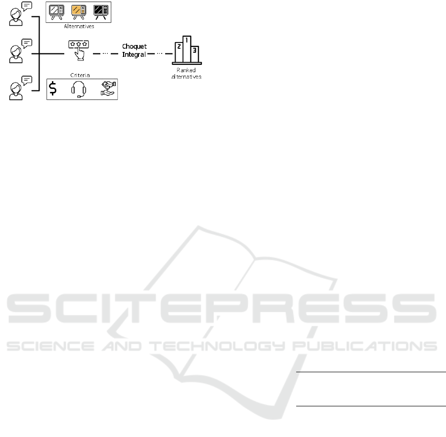
Figure 1: Image description of the decision making process

using the Choquet integral. Source: the authors.

To describe the GMC-RTOPSIS method let q rep-

resent the q-th decision maker in a collection of

Q ∈ N = {1,2, 3,...} ones. Let A

A = {A

,..., A

}

be the set of alternatives for the problem and C

,...,C

} represent the criteria set for decision

maker q. With C

C = {C

,...,C

} = {C

,...,C

where n =

∑

q=1

, representing the criteria set of all

the decision makers. From these notations we can

represent each of the q-th decision maker by the ma-

trix below (Eq. (3)), called decision matrix DM:







··· C

) s

) ··· s

)

) s

) ··· s

)

) s

) ··· s

)







(3)

Each matrix cell s

i j

), with 1 ≤ i ≤m, 1 ≤ j ≤ n

is called the rating of the criterion j for alternative

i. Also, notice that the rating is a function of Y

Y =

rand

, Y

det

), which are factors that model random

and deterministic events. Random events are modeled

by stochastic processes, and deterministic are events

which are not random, like time, location or a param-

eter of a random event. A ﬁxed value x of the deter-

ministic vector is called a state, and the set of all states

is represented by X .

In possession of all decision matrices from all

decision-makers Q, the algorithm can be applied. The

process is quite similar to the original TOPSIS, pre-

sented in 1981. It uses the same deﬁnition of Posi-

tive Ideal Solution (PIS) and Negative Ideal Solution

(NIS) that are, respectively, the one that is closer to

the best possible solution and the one that is distant

from the best possible solution, see Eq. (4). The

most signiﬁcant difference is that each criterion may

use a different distance measure since each may have

its own type. So, the distances of each criterion are

calculated separately and aggregated afterward in the

separation measure step of the algorithm (see Figure

2).

In order to ease the comprehension of our ap-

proach, we present in Figure 2 the steps of the GMC-

RTOPSIS, where:

Step 0. Select a state x ∈ X not yet processed;

Step 1. Normalize all matrices;

Step 2. Select the PIS, denoted by s

Y ), and

the NIS, denoted by s

−

Y ), considering, for each

j ∈ {1,. ..,n}, respectively:

Y ) =







max

1≤i≤m

i j

, if it is a beneﬁt criterion,

min

1≤i≤m

i j

if it is a cost/loss criterion,

(4)

−

Y ) =







min

1≤i≤m

i j

, if it is a beneﬁt criterion,

max

1≤i≤m

i j

, if it is a cost/loss criterion;

Step 3. Calculate the distance measure for each

criterion C

, with j ∈ {1,..., n}, to the PIS and

NIS solutions, that is,

i j

= d(s

Y ), s

i j

Y )),

−

i j

= d(s

−

Y ), s

i j

Y )),

where i ∈ {1,. .. ,m} and d is a distance measure

associated with the criteria data type;

Step 4. Calculate the separation measure, for each

i ∈ {1,. .. ,m}, using the Choquet integral as fol-

lows:

Y ) =

∑

j=1





i( j)



−



i( j−1)





( j)

)

−

Y ) =

∑

j=1





−

i( j)



−



−

i( j−1)





−

( j)

)

where d

i(1)

≤ . .. ≤ d

i(n)

, d

−

i(1)

≤ . .. ≤ d

−

i(n)

, for

each j ∈ {1,... ,n}, C

( j)

is the criterion cor-

respondent to d

i( j)

, C

−

( j)

is the criterion corre-

spondent to d

−

i( j)

, C

( j)

= {C

( j)

( j+1)

,...,C

(n)

−

( j)

= {C

−

( j)

−

( j+1)

,...,C

−

(n)

}, C

(n+1)

= C

−

(n+1)

0, d

i(0)

= d

−

i(0)

= 0 and m

is the learned fuzzy

measure by a particle swarm optimization algo-

rithm (Wang et al., 2011).

Here, the separation measure is the square root of

the Choquet integral of squared distances, and this

means that it is the square root of a d-Choquet in-

tegral (Bustince et al., 2020). Also, for each state,

we may have a different fuzzy measure, which

means that the fuzzy measure is dependent on Y

det

CC-separation Measure Applied in Business Group Decision Making

455

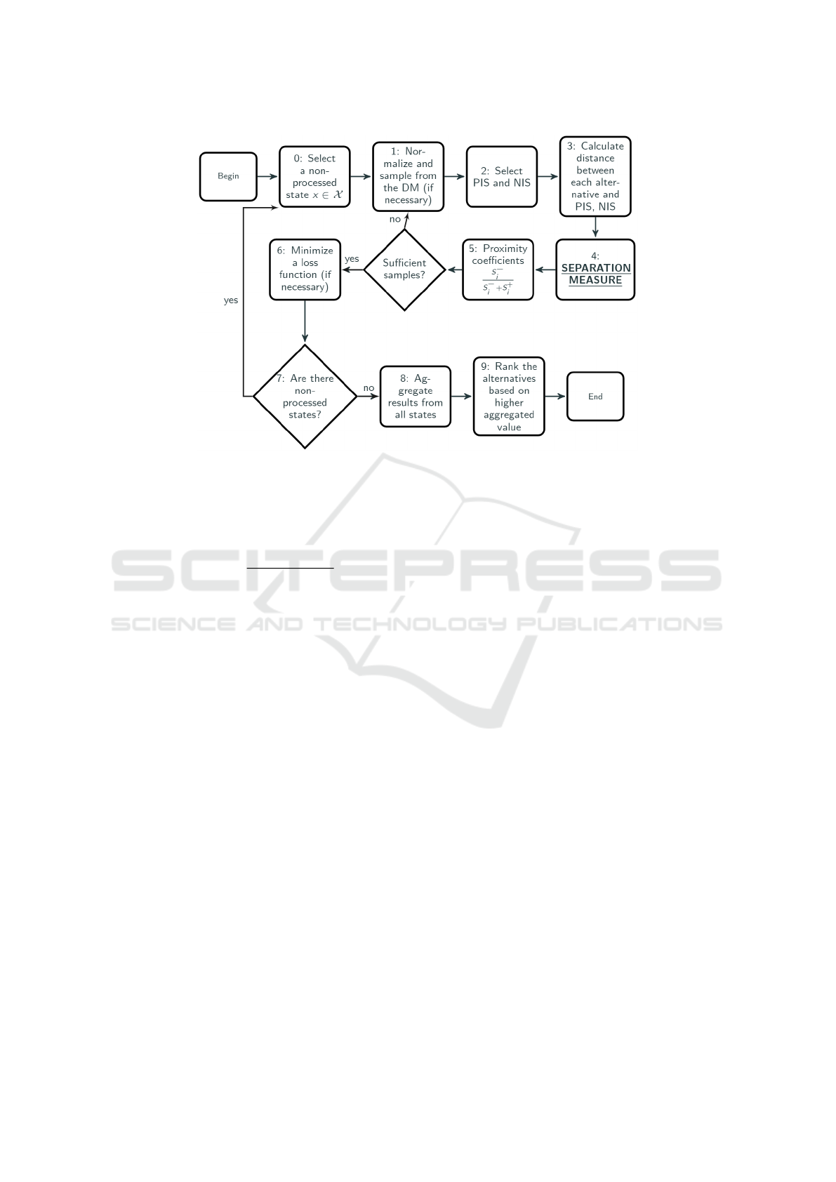
Figure 2: Diagram of the GMC-RTOPSIS process. The separation measure step is where the CC-separation measure is used.

Source: The authors.

Step 5. For each i ∈ {1,..., m}, calculate the

relative closeness coefﬁcient to the ideal solution

with:

Y ) =

−

Y )

−

Y ) + S

Y )

;

Step 6. By using probability distributions in the

DM, it is introduced a bootstrapped probability

distribution in the CC

values, so as a point repre-

sentation for this distribution we minimize a pre-

deﬁned risk function:

= argmin

R(c)

= argmin

L(c, CC

Y )) dF(CC

Y )); (5)

Step 7. If there is at least one non-processed state

x, return to Step 0;

Step 8. Aggregate the cc

values from all the

states with

= f

x∈X

(cc

(x)), where f is an ag-

gregation function.

Step 9. Finally, rank the alternatives from the

highest to the lowest

values.

3 GENERALIZATION OF THE

GMC-RTOPSIS BY USING

CC-INTEGRALS

Using the Choquet integral in the separation mea-

sure, the GMC-RTOPSIS method allows for interac-

tion among different criteria. This is the step where

this study incorporates the CC-integrals in place of

the Choquet integral.

We introduce the CC-separation measure by:

Deﬁnition 3.1 (CC-separation measure). Let Co be

a bivariate copula and m a fuzzy measure. A CC-

separation measure S

∗

: [0,1]

→ [0,1] is deﬁned, for

all i ∈ {1,. .. ,m}, by the functions:

Y ) =

∑

j=1





i( j)



, m



( j)





−Co





i( j−1)



, m



( j)





1/2

−

Y ) =

∑

j=1





−

i( j)



, m



−

( j)





−Co





−

i( j−1)



, m



−

( j)





1/2

where d

i( j)

, d

−

i( j)

, C

( j)

, C

−

( j)

and m

are deﬁned as in

Step 4 of the GMC-RTOPSIS algorithm. Note that

the separation measure is the squared root of the CC-

integral, which is an aggregation function as shown

in (Lucca et al., 2017a).

ICEIS 2021 - 23rd International Conference on Enterprise Information Systems

456

4 EXPERIMENTAL

FRAMEWORK

In this section, we present the application of the CC-

separations in the GMC-RTOPSIS. To do so, we start

describing the methodology adopted in the study; af-

ter that, the example in which we apply our approach

is described, and lastly, the obtained results are pre-

sented and discussed.

4.1 Methodology

In this study, we will apply the proposed CC-

separation measure to the Case Study 2 introduced

in (Lourenzutti et al., 2017) and used in (Wieczyn-

ski et al., 2020) to ease the comparison between the

different CC-integrals.

To perform the simulation, we used 10,000 sam-

ples from the DM. We also applied a particle swarm

optimization to learn the fuzzy measure using 30 par-

ticles and 100 interactions. The PSO is used since the

original method had good outcomes with the method.

In this study we used the copula functions from

Table 1. We highlight that we used 2 different values

for the α parameter, which are α = 0.1, selected from

the literature (Lucca et al., 2017a), and α = 0.6, which

was the best ﬁt for the problem presented in this paper

based on the difference between the ﬁrst and second

ranked alternatives, when compared to other α values.

For the risk function, given in Eq. (5), it was used

the squared loss:

L(cc, CC

) = (cc −CC

)

This result in the mean function being the point esti-

mator for the process.

Also, we use the aggregation function bellow in

the Step 8 of the algorithm:

WAM

= w(S

) ·cc

) + w(S

) ·cc

For the analysis of the results from the different cop-

ula functions, we use the difference between the alter-

native ranked ﬁrst to the second ranked with:

∆

R1,R2

= max ( ˆc

) −max ( ˆc

)

where ˆc

= {cc

| i ∈ {1,.. ., m}} and ˆc

= ˆc

−

{max( ˆc

)}.

Lastly, since we are altering only the Choquet

function, the algorithm maintains its original com-

plexity.

4.2 The Considered Problem

A company needs a new supplier for a provision and

is evaluating four different suppliers, namely A

, A

and A

. The company called three of its managers

to analyze the suppliers and give their ratings based

on their criteria.

The ﬁrst manager is a budget manager. He con-

sidered the price per batch (in thousands) as C

(1)

warranty (in days) as C

(1)

and payment conditions

(in days) as C

(1)

. Also, it was considered that the

demand for the product is higher in December. He

modeled it by using a binary variable τ, that is τ = 0

when the month is between January and November,

and τ = 1 when it is December. Finally, he assigned a

weight for each of his criterion with a weighting vec-

tor: w

(1)

= (0.5, 0.25, 0.25).

The second manager, a product manager, consid-

ered the price as C

(2)

, delivery time (in hours) as C

(2)

production capacity C

(2)

, product quality C

(2)

and the

time to respond to a support request (in hours) as

(2)

. Additionally, to account for the reliability in the

production process and what a failure in the process

could cause to the supplier’s production capacity, he

let P

be a random variable such that P

= 0 occurs

when there are no failures in the production process

of the supplier A

, and P

= 1 when there are fail-

ures. Also, in December, the production is acceler-

ated, so the chance of failure is higher, so he modeled

a stochastic process with the help of the function:

(x,y) = x



1 + y(P

+ τ)



Lastly, the production capacity was modeled by using

ITFNs:



(0.8

1+P

,0.9

1+P

,1.0

1+P

,1.0

1+P

), 1.0, 0.0





(0.8

1+4P

,0.9

1+4P

,1.0

1+4P

,1.0

1+4P

), 0.7, 0.1





(0.6

1+2P

,0.7

1+2P

,0.8

1+2P

,1.0

1+2P

), 0.8, 0.0





(0.5

1+3P

,0.6

1+3P

,0.8

1+3P

,0.9

1+3P

), 0.8, 0.1



This manager selected the same weight for all criteria,

i.e w

(2)

= (0.2, 0.2, 0.2, 0.2, 0.2).

The commercial manager was the third. He con-

sidered the product lifespan (in years) as C

(3)

, social

and environmental responsibility as C

(3)

, the quan-

tity of quality certiﬁcations as C

(3)

and the price as

(3)

. The weighting vector provided by this manager

is w

(3)

= (0.25, 0.12, 0.23, 0.4).

The P

distribution was determined by historical

data of each supplier and it is given as follows:

• For τ = 0:

p(P

= 0|S

) = 0.98,

p(P

= 0|S

) = 0.96,

p(P

= 0|S

) = 0.97,

p(P

= 0|S

) = 0.95.

CC-separation Measure Applied in Business Group Decision Making

457

Table 1: Examples of Copulas.

(I) T-norms

Deﬁnition Name/Description

(x,y) = min{x,y} Minimum

(x,y) = xy Algebraic Product

(x,y) = max{0,x + y −1} Łukasiewicz

(x,y) =

(

min{x, y} if x + y > 1

0 otherwise

Nilpotent Minimum

(x,y) =

(

0 if x = y = 0

x+y−xy

otherwise

Hamacher Product

(II) Non-associative overlap functions

Deﬁnition Reference/Description

(x,y) = min{x

√

y,y

√

x} Cuadras-Aug

e family of copulas (Nelsen, 2007)

(x,y) = min{x,y}max{x

} (Dimuro and Bedregal, 2014; Pereira Dimuro et al., 2016)

(x,y) = xy(1 + α(1 −x)(1 −y)),

where α ∈ [−1,0[ ∪ ]0,1]

(Alsina et al., 2006; Lucca et al., 2015)

(III) Non-associative copulas, which are neither t-norms nor overlap functions

Deﬁnition Reference/Description

(x,y) = xy + x

y(1 −x)(1 −y) (Klement et al., 2011)

(x,y) = max{min{x,

},x + y −1} (Alsina et al., 2006)

Div

(x,y) =

xy+min{x,y}

(Alsina et al., 2006)

• For τ = 1:

p(P

= 0|S

) = 0.96,

p(P

= 0|S

) = 0.92,

p(P

= 0|S

) = 0.96,

p(P

= 0|S

) = 0.90.

Considering all the DMs, we have the following

underlying factors: a random component Y

rand

) and a deterministic component Y

det

= τ

that has two states: S

when τ = 0 and S

when

τ = 1. The underlying factors can be represented by

Y = (Y

rand

, Y

det

). The managers agreed that the state

was more important, since the production is higher,

so they gave it a higher weight for it in the aggregation

step (Step 8 of the method) by setting w(S

) = 0.4 and

w(S

) = 0.6.

The DMs of all managers are presented in Table

2, where the linguistic variables (W, P, I, G and E) are

deﬁned as in Table 3.

The company, considering the opinion of manager 2

more important, assigned a weighting vector for the

managers represented by w

w = (0.3, 0.4, 0.3). Fur-

thermore, they wanted to include some interaction be-

tween the criteria, so a variation of 30% was allowed

for each fuzzy measure in relation to the coefﬁcient

in the additive fuzzy measure. This measure is calcu-

lated computationally by means of the PSO algorithm

(Wang et al., 2011; Lourenzutti et al., 2017).

4.3 Obtained Results

The aggregated ranked results are presented in Table 4

(for all the results see APPENDIX Table 5). The table

shows for each copula function Co, the rank of alter-

natives from columns 2 to 5, with its aggregated val-

ues inside parenthesis. The last column shows the dif-

ference between alternatives ranked ﬁrst and ranked

second.

We can see that for the t-norms the values are pro-

ICEIS 2021 - 23rd International Conference on Enterprise Information Systems

458

Table 2: Decision matrices for the managers.

(a) Budget manager

Alternatives C

(1)

τ = 0 τ = 1

260.00(1 + 0.15τ) 90 G G

250.00(1 + 0.25τ) 90 P W

350.00(1 + 0.20τ) 180 G I

550.00(1 + 0.10τ) 365 I W

(b) Production manager

Alternatives C

(2)

260.00 U( f

(48, 0.10), f

(96, 0.10)) s

I [24, 48]

250.00 U( f

(72, 0.20), f

(120, 0.20)) s

P [24, 48]

350.00 U( f

(36, 0.15), f

(72, 0.15)) s

G [12, 36]

550.00 U( f

(48, 0.25), f

(96, 0.25)) s

E [0, 24]

Alternatives C

(3)

Exp(3.5) W 1 260.00

Exp(3.0) W 0 250.00

Exp(4.5) P 3 350.00

Exp(5.0) I 5 550.00

Table 3: Linguistic variables and their respective trape-

zoidal fuzzy numbers.

Linguistic variables Trapezoidal fuzzy numbers

Worst (W) (0, 0, 0.2, 0.3)

Poor (P) (0.2, 0.3, 0.4, 0.5)

Intermediate (I) (0.4, 0.5, 0.6, 0.7)

Good (G) (0.6, 0.7, 0.8, 1)

Excellent (E) (0.8, 0.9, 1, 1)

portional to the ones presented in the study that used

-integral instead of the Choquet integral (Wieczyn-

ski et al., 2020). As in that paper, here the T

t-norm

has the greatest difference, with ∆

R1, R2

= 0.0700. Al-

though, only the T

t-norm performs well compared

with other copulas such as O

and C

The copula O

with α = 0.6 achieved the sec-

ond greatest difference among the tested ones, with

∆

R1, R2

= 0.0502. The next of this family tested was

the one with α = 0.1, as it is the main value used in the

literature, it resulted in a quite lower difference value,

with only ∆

R1, R2

= 0.0294. Among the copulas from

the α family, we have C

, with ∆

R1, R2

= 0.0466 and

with ∆

R1,R2

= 0.0454.

Notice that when using C

div

, C

and T

copulas the

alternatives A

and A

change position. This is from

the inﬂuence of the state 2 result, where these func-

tions may have weighted higher criteria for alternative

. Furthermore, the relative small difference ∆

R1,R2

make the top of the rank prone to invert positions.

Our last analysis considered the CC-separations

that presented the lowest ranks. Precisely, it is

observable in the obtained results that the copulas

and T

obtained a similar performance

and the lowest separation.

5 CONCLUSIONS

The GMC-RTOPSIS is a decision method that

chooses the alternative that is closer to an ideal solu-

tion. It is capable of dealing with multiple data types

as inputs and, also, through the Choquet integral, con-

siders the interaction among different criteria.

In this paper, we presented the CC-separation

measure. A new measure to be used in the GMC-

RTOPSIS method that utilizes the CC-integrals in-

stead of the Choquet integral. The CC-integrals is a

generalization of the Choquet integral that presented

CC-separation Measure Applied in Business Group Decision Making

459

Table 4: Rank of the alternatives with each of the C functions, ordered by difference between the value of the alternative

ranked ﬁrst and second.

Co function Ranked 1st Ranked 2nd Ranked 3rd Ranked 4th ∆

R1,R2

(0.6462) A

(0.5762) A

(0.4616) A

(0.3782) 0.0700

α=0.6

(0.5897) A

(0.5395) A

(0.4716) A

(0.4282) 0.0502

(0.5991) A

(0.5525) A

(0.4453) A

(0.4194) 0.0466

(0.5919) A

(0.5493) A

(0.4713) A

(0.3910) 0.0425

α=0.1

(0.5953) A

(0.5659) A

(0.4453) A

(0.3962) 0.0294

(0.5995) A

(0.5715) A

(0.4454) A

(0.3927) 0.0280

Div

(0.5234) A

(0.5016) A

(0.4868) A

(0.4250) 0.0218

(0.5273) A

(0.5097) A

(0.4914) A

(0.4361) 0.0176

(0.5351) A

(0.5221) A

(0.5049) A

(0.4308) 0.0131

(0.5821) A

(0.5701) A

(0.4346) A

(0.3977) 0.0120

(0.5511) A

(0.5395) A

(0.4713) A

(0.4133) 0.0116

(0.5229) A

(0.5118) A

(0.4737) A

(0.4386) 0.0110

good results when applied in classiﬁcation problems.

By using an example from the literature, we tested

the method with 11 different copula functions, with

one of them using two distinct parameters. The re-

sults indicate that the Łukasiewicz t-norm is the best

copula function to use in this example problem since

it gives the greatest separation between the alterna-

tives ranked ﬁrst and second. Additionally, the Over-

lap alpha family, with α = 0.6, the C

and the T

also presented good separations.

By being able to verify the separation between the

ranks, we can choose more conﬁdently the alternative

that better suits the problem. Therefore, by using mul-

tiple functions in the CC-separation measure, we can

see how the problem behaves in different situations.

Finally, future work will consider learning the α

parameter of the overlap alpha family, using distinct

optimization methods.

ACKNOWLEDGMENTS

We would like to thank Dr. Helida S. San-

tos for reviewing the text. This study was sup-

ported by PNPD/CAPES (464880/2019-00) and

CAPES Financial Code 001, CNPq (301618/2019-4),

FAPERGS (19/2551-0001279-9, 19/ 2551-0001660)

and, the Spanish Ministry of Science and Tech-

nology (PC093-094TFIPDL, TIN2016-81731-REDT,

TIN2016-77356-P (AEI/FEDER, UE)).

REFERENCES

Alazzawi, A. and

Zak, J. (2020). Mcdm/a based design

of sustainable logistics corridors combined with sup-

pliers selection. the case study of freight movement

to iraq. Transportation Research Procedia, 47:577 –

584. 22nd EURO Working Group on Transportation

Meeting, EWGT 2019, 18th – 20th September 2019,

Barcelona, Spain.

Alsina, C., Frank, M. J., and Schweizer, B. (2006). As-

sociative Functions: Triangular Norms and Copulas.

WORLD SCIENTIFIC.

Bustince, H., Fernandez, J., Mesiar, R., Montero, J., and Or-

duna, R. (2010). Overlap functions. Nonlinear Anal-

ysis, 72:1488–1499.

Bustince, H., Mesiar, R., Fernandez, J., Galar, M., Pater-

nain, D., Altalhi, A., Dimuro, G., Bedregal, B., and

Takac, Z. (2020). d-choquet integrals: Choquet inte-

grals based on dissimilarities. Fuzzy Sets and Systems.

(submitted).

Candeloro, D., Mesiar, R., and Sambucini, A. R. (2019). A

special class of fuzzy measures: Choquet integral and

applications. Fuzzy Sets and Systems, 355:83 – 99.

Theme: Generalized Integrals.

Choquet, G. (1953–1954). Theory of capacities. Annales

de l’Institut Fourier, 5:131–295.

Deveci, M., C¸ etin Demirel, N., and Ahmeto

glu, E. (2017).

Airline new route selection based on interval type-

2 fuzzy mcdm: A case study of new route between

turkey- north american region destinations. Journal of

Air Transport Management, 59:83 – 99.

Dimuro, G. P. and Bedregal, B. (2014). Archimedean over-

lap functions: The ordinal sum and the cancellation,

idempotency and limiting properties. Fuzzy Sets and

Systems, 252:39 – 54. Theme: Aggregation Functions.

ICEIS 2021 - 23rd International Conference on Enterprise Information Systems

460

Dimuro, G. P., Fern

andez, J., Bedregal, B., Mesiar, R.,

Sanz, J. A., Lucca, G., and Bustince, H. (2020). The

state-of-art of the generalizations of the choquet in-

tegral: From aggregation and pre-aggregation to or-

dered directionally monotone functions. Information

Fusion, 57:27 – 43.

Dimuro, G. P., Lucca, G., Sanz, J. A., Bustince, H., and

Bedregal, B. (2018). Cmin-integral: A choquet-like

aggregation function based on the minimum t-norm

for applications to fuzzy rule-based classiﬁcation sys-

tems. In Torra, V., Mesiar, R., and Baets, B. D., ed-

itors, Aggregation Functions in Theory and in Prac-

tice, pages 83–95, Cham. Springer International Pub-

lishing.

Grabisch, M., Marichal, J.-L., Mesiar, R., and Pap, E.

(2009). Aggregation Functions. page 480.

Huang, C. and Yoon, K. (1981). Multiple Attribute Deci-

sion Making: Methods and Applications. A State-of-

the-Art Survey. Number 186 in Lecture Notes in Eco-

nomics and Mathematical Systems. Springer, Berlin,

Heidelberg.

Klement, E. P., Mesiar, R., and Pap, E. (2011). Triangu-

lar Norms. Springer, Dordrecht; London. OCLC:

945924583.

Lourenzutti, R., Krohling, R. A., and Reformat, M. Z.

(2017). Choquet based TOPSIS and TODIM for dy-

namic and heterogeneous decision making with crite-

ria interaction. Information Sciences, 408:41–69.

Lucca, G., Dimuro, G. P., Mattos, V., Bedregal, B.,

Bustince, H., and Sanz, J. A. (2015). A family of

Choquet-based non-associative aggregation functions

for application in fuzzy rule-based classiﬁcation sys-

tems. In 2015 IEEE International Conference on

Fuzzy Systems (FUZZ-IEEE), pages 1–8, Los Alami-

tos. IEEE.

Lucca, G., Sanz, J. A., Dimuro, G. P., Bedregal, B., Asi-

ain, M. J., Elkano, M., and Bustince, H. (2017a).

CC-integrals: Choquet-like Copula-based aggrega-

tion functions and its application in fuzzy rule-based

classiﬁcation systems. Knowledge-Based Systems,

119:32–43.

Lucca, G., Sanz, J. A., Dimuro, G. P., Bedregal, B.,

Fern

andez, J., and Bustince, H. (2017b). Analyzing

the behavior of a CC-integral in a fuzzy rule-based

classiﬁcation system. In 2017 IEEE International

Conference on Fuzzy Systems (FUZZ-IEEE), pages 1–

6, Los Alamitos. IEEE.

Lucca, G., Sanz, J. A., Dimuro, G. P., Bedregal, B.,

Mesiar, R., Kolesarova, A., and Bustince, H. (2016).

Preaggregation Functions: Construction and an Ap-

plication. IEEE Transactions on Fuzzy Systems,

24(2):260–272.

Mesiar, R. and Stup

nanov

a, A. (2019). A note on cc-

integral. Fuzzy Sets and Systems, 355:106 – 109.

Theme: Generalized Integrals.

Murofushi, T. and Sugeno, M. (1989). An interpretation

of fuzzy measures and the choquet integral as an inte-

gral with respect to a fuzzy measure. Fuzzy Sets and

Systems, 29(2):201 – 227.

Nelsen, R. B. (2007). An introduction to copulas. Springer

Science & Business Media.

Pereira Dimuro, G., Bedregal, B., Bustince, H., Asi

ain,

M. J., and Mesiar, R. (2016). On additive generators

of overlap functions. Fuzzy Sets and Systems, 287:76

– 96. Theme: Aggregation Operations.

Shyur, H.-J. and Shih, H.-S. (2006). A hybrid mcdm

model for strategic vendor selection. Mathematical

and Computer Modelling, 44(7):749 – 761.

Sugeno, M. (1974). Theory of Fuzzy Integrals and its Ap-

plications. PhD thesis, Tokyo Institute of Technology,

Tokyo.

Wang, X.-Z., He, Y.-L., Dong, L.-C., and Zhao, H.-Y.

(2011). Particle swarm optimization for determin-

ing fuzzy measures from data. Information Sciences,

181(19):4230–4252.

Wieczynski, J. C., Dimuro, G. P., Borges, E. N., Santos,

H. S., Lucca, G., Lourenzutti, R., and Bustince, H.

(2020). Generalizing the GMC-RTOPSIS method us-

ing CT-integral pre-aggregation functions. In 2020

IEEE International Conference on Fuzzy Systems

(FUZZ-IEEE), pages 1–8, Glasgow.

Zadeh, L. A. (1965). Fuzzy sets. Information and Control,

8(3):338–353.

CC-separation Measure Applied in Business Group Decision Making

461

APPENDIX

Table 5: Mean and standard deviation of the alternatives for

State 1 and State 2. The highest mean for each function and

state is in boldface and the highest for the criterion has an

asterisk*.

State 1 (S

, τ = 0) State 2 (S

, τ = 1)

Alternatives A

Function mean std.dev mean std.dev mean std.dev mean std.dev mean std.dev mean std.dev mean std.dev mean std.dev

0.4702 0.0482 0.4360 0.0116 0.6438* 0.0367 0.5588 0.0119 0.4558 0.0506 0.3397 0.0334 0.6478* 0.0477 0.5878* 0.0250

α=0.6

0.4852 0.0134 0.4791* 0.0232 0.5742 0.0731 0.5078 0.0108 0.4625 0.0266 0.3943 0.0165 0.6001 0.0593 0.5607 0.0214

0.4774 0.0181 0.4604 0.0173 0.6074 0.0858 0.5270 0.0135 0.4239 0.0194 0.3921 0.0208 0.5935 0.0710 0.5695 0.0174

0.4643 0.0269 0.4276 0.0178 0.5939 0.0469 0.5654 0.0186 0.4759 0.0399 0.3666 0.0362 0.5905 0.0379 0.5386 0.0368

α=0.1

0.4568 0.0127 0.4282 0.0117 0.6013 0.0791 0.5656 0.0098 0.4377 0.0275 0.3749 0.0223 0.5913 0.0611 0.5661 0.0232

0.4519 0.0134 0.4218 0.0171 0.6119 0.0772 0.5668 0.0156 0.4411 0.0308 0.3733 0.0150 0.5912 0.0789 0.5746 0.0271

Div

0.5100 0.0101 0.4654 0.0187 0.5139 0.0202 0.5221 0.0191 0.4713 0.0293 0.3980 0.0088 0.4934 0.0242 0.5242 0.0307

0.5251* 0.0082 0.4670 0.0144 0.5335 0.0058 0.5242 0.0126 0.4690 0.0427 0.4155 0.0165 0.4938 0.0186 0.5293 0.0314

0.4976 0.0083 0.4648 0.0141 0.5328 0.0169 0.5253 0.0125 0.5097* 0.0198 0.4081 0.0114 0.5367 0.0207 0.5199 0.0157

0.4567 0.0120 0.4270 0.0093 0.5976 0.0655 0.5674* 0.0098 0.4198 0.0396 0.3782 0.0190 0.5718 0.0605 0.5719 0.0360

0.4843 0.0148 0.4443 0.0138 0.5584 0.0422 0.5487 0.0101 0.4626 0.0360 0.3926 0.0156 0.5462 0.0388 0.5334 0.0306

0.4701 0.0478 0.4615 0.0217 0.5326 0.0018 0.5279 0.0231 0.4761 0.0270 0.4234* 0.0232 0.4980 0.0087 0.5195 0.0269

ICEIS 2021 - 23rd International Conference on Enterprise Information Systems

462