Water Hazard Depth Estimation for Safe Navigation of Intelligent

Vehicles

Zoltan Rozsa

1,2 a

, Marcell Golarits

1 b

and Tamas Sziranyi

1,2 c

Machine Perception Research Laboratory of Institute for Computer Science and Control (SZTAKI), E

otv

os Lor

and

Research Network (ELKH), H-1111 Budapest, Kende u. 13-17, Hungary

Faculty of Transportation Engineering and Vehicle Engineering, Budapest University of Technology and Economics

(BME-KJK), H-1111 Budapest, M

uegyetem rkp. 3, Hungary

Keywords:

Intelligent Vehicles, Machine Vision, Point Cloud Processing, Plane Fitting, Segmentation, Multi-media

Photogrammetry.

Abstract:

This paper proposes a method to provide depth information about water hazards for ground vehicles. We can

estimate underwater depth even with a moving mono camera. Besides the physical principles of refraction,

the method is based on the theory of multiple-view geometry and basic point cloud processing techniques. We

use the information gathered from the surroundings of the hazard to simplify underwater shape estimation.

We detect water hazards, estimate its surface and calculate real depth of underwater shape based on matched

points using refraction principle. Our pipeline was tested on real-life experiments, on-board cameras and a

detailed evaluation of the measurements is presented in the paper.

1 INTRODUCTION

There are scenarios where water depth needs to be es-

timated, but the camera is the only viable sensor op-

tion. For example, it is not worth using speciﬁc sen-

sors; using active sensors should be avoided (Rankin

and Matthies, 2010), or simply because installing dif-

ferent kinds of sensors is not possible (for example, to

an UAV - Unmanned Aerial Vehicle). Also, solving

the problem with cameras can be a relatively cheap

solution or increase the redundancy (and the reliabil-

ity) of the whole system applying together with other

sensors.

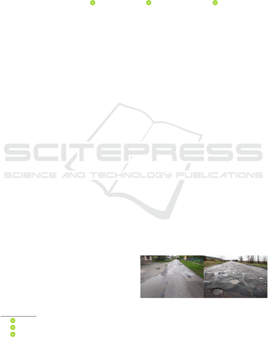
We propose to apply the proposed method in au-

tonomous driving (or driver assistance) in an off-road

(or on-road with potholes, Figure 1) environment.

During or after heavy raining the probability of ac-

cidents increases (Song. et al., 2020). Puddles can

form, which depth needs to be estimated to decide

whether the vehicle can wade through safely the water

or search for a bypass route.

Bathymetric (the discipline of determining the

depth of the ocean or lake ﬂoors) mapping is usu-

https://orcid.org/0000-0002-3699-6669

https://orcid.org/0000-0001-9652-4148

https://orcid.org/0000-0003-2989-0214

ally done with speciﬁc active equipment like SoNAR

or LIDAR (Costa et al., 2009). Recently, to con-

struct Digital Elevation Models (DEMs), satellite and

UAV (Unmanned Aerial Vehicle) images are also ap-

plied in shallow water bathymetry. These methods (as

shown later) apply simpliﬁcations of the problem due

to the high-altitude imaging. However, in the case of

ground vehicles, the incidence ray going the camera

is not close to being perpendicular to the water sur-

face in general. (As this would require the vehicle to

be above the water surface.) Our correction solution

is deﬁned in a general coordinate system for general

vehicle (and camera) pose, which has not been done

before.

(a) Own photograph (b) Source: www.totalcar.hu

Figure 1: Illustration of roads with potholes after raining.

We propose a pipeline to get a deterministic so-

lution of the depth in an underwater surface with a

Rozsa, Z., Golarits, M. and Sziranyi, T.

Water Hazard Depth Estimation for Safe Navigation of Intelligent Vehicles.

DOI: 10.5220/0010438100900099

In Proceedings of the 7th International Conference on Vehicle Technology and Intelligent Transport Systems (VEHITS 2021), pages 90-99

ISBN: 978-989-758-513-5

mono camera above the water. The workﬂow can be

used with a stereo camera pair or a mono camera (in

case of correct scaling) as well. We will show exam-

ples for both cases. In the stereo case, the absolute

scaling is given and we have a stereo reconstruction

problem, while in the mono camera case we deal with

the Structure from Motion (SfM) problem.

1.1 Contributions

The paper contributes to the following:

• Novel methodology is proposed to estimate water

depth with a mono (or stereo) camera.

• Basic refraction theory of optics is combined with

geometry-based point cloud processing.

• There are no restrictions to camera (vehicle) pose.

Besides the theory, practical applications are shown,

and evaluation is presented about the proposed

method’s performance.

1.2 Outline of the Paper

The paper is organized as follows: Section 2 sur-

veys the literature about the related works. Section

3 describes the proposed pipeline in detail. Section

4 shows our test results and Section 5 discuss them.

Finally, Section 6 draws the conclusions.

2 RELATED WORKS

For autonomous navigation or ADAS (Advanced

Driver Assistance System) purposes, researches deal-

ing with water hazard detection has a relatively long

history, papers related to this topic were ﬁrst pub-

lished more than a decade ago (Xie et al., 2007).

Since than there were numerous solution proposed

to this problem based on handcrafted features from

texture and color (Zhao et al., 2014), spatio-temporal

features (Mettes et al., 2017), MRF (Haris and Hou,

2020) models, polarization (Nguyen et al., 2017) or

active sensors (Chen et al., 2017). The current state

of the art employes deep learning techniques for this

task (Han et al., 2018), (Qiao et al., 2020). So there

is a wide range of solutions for the detection task. We

go further, and improve the detection with water depth

estimation.

The detection can result in an avoid (if it is pos-

sible) or slow down command, but as the depth of

the hazard is unknown, the degree of deceleration

required (to maintain the vehicle’s and passengers’

health) is unknown. In an off-road environment, the

consequences of traversing through a water hazard (at

a given speed) can be even more extreme, and the de-

cision even more critical. For example, the traversable

path of an off-road vehicle can be crossed with a

brooklet. The depth of the brooklet (can be much

deeper than a pothole ﬁlled with water) must be care-

fully assessed, as ﬁnding a pass through the booklet

can be very time consuming, but wading through it

may cause severe damage to the mechanic and elec-

tronic parts of the vehicle. That is why we propose a

method to estimate the (real) depth of still water based

on vision.

The problems of multi-medium photogrammetry

is an interest of computer vision and geodesy com-

munity for decades (Fryer, 1983) (Shan, 1994). The

century advancement of the topic related to com-

puter vision is mainly based on the theory of (Agrawal

et al., 2012) and (Chari and Sturm, 2009). The ﬁrst

ones state that the n-layer ﬂat refraction system cor-

responds to an axial camera. The second one lays the

foundation for determining fundamental matrices in

the presence of refraction.

Recent literature primarily related to machine vi-

sion in this topic mostly tries to estimate relative cam-

era motion and build the structure from motion model

from underwater images (Kang et al., 2012) (Jordt-

Sedlazeck and Koch, 2013). Instead of doing that, we

will use the reconstruction of the shore environment,

which is not affected by the refraction. Besides, (Mu-

rai et al., 2019) uses a multi-wavelength camera to re-

construct surface normals, and (Qian et al., 2018) pro-

posed a method to reconstruct the water surface with

the underwater scene simultaneously. They used four

cameras, which makes the application hard in prac-

tice.

Results rather related to bathymetry are closer to

the practical application (Terwisscha van Scheltinga

et al., 2020) of multi-medium photogrammetry, as in

most cases are trying to minimize the effect of refrac-

tion in depth estimation. The bathymetry researches

below are the most related to our work, but they

cannot be compared to ours as they examine com-

pletely different water areas in completely different

circumstances. As they use high altitude images, of-

ten signiﬁcant simpliﬁcations are made (e.g., the un-

derwater depth and camera height ratio is negligible,

ray direction is approximately perpendicular to the

water surface) (Dietrich, 2017) or parameters gener-

ally unknown are used for the calculation (e.g., sea

level from GPS data) (Agraﬁotis et al., 2020). Re-

fraction can be corrected analytically (Maas, 2015)

or iteratively (Skarlatos and Agraﬁotis, 2018) with

prior knowledge. In recent research, (Agraﬁotis et al.,

2019) machine learning technique was also applied to

correct the refraction.

Water Hazard Depth Estimation for Safe Navigation of Intelligent Vehicles

The advantages of our proposed method compared

to the literature:

• We solve the problem in a general coordinate sys-

tem. This way, simpliﬁcations (comes from cam-

era pose and motion) are not necessary.

• Extra or speciﬁc sensors are not required.

• The solution can be determined explicitly.

3 THE PROPOSED METHOD

There are a few features of water hazards, which we

utilize in the paper:

• The water in them is approximately still, so its sur-

face is considered to be planar in the examined

area. (We do not consider wave effects like (Fryer

and Kniest, 1985).)

• The hazards are surrounded by road or traversable

path; thus, we do not need underwater SfM.

Ground parts of the images can be used for rela-

tive camera motion estimation. Note: This is only

important in the mono camera case, as, in the case

of stereo camera rig, the relative pose of the cam-

eras is known.

The proposed pipeline can be divided into the follow-

ing main steps:

1. Preprocessing (From calibration to detection of

water hazards)

2. Estimating water surface (plane ﬁtting in the cam-

era coordinate system) in order to ﬁnd ray-surface

intersection point

3. Calculating underwater depth (Triangulation and

correction based on Snell’s law)

3.1 Preprocessing

In the following, we will indicate the preprocessing

steps for both mono and stereo camera cases. Note:

We designed our method to be able to work with us-

ing only a single camera (and a stereo camera rig as

well). However, in a real-time application, we suggest

applying the stereo camera solution (as it simpliﬁes

the problem.) Mono camera solution is important in

this case too, to increase the reliability of the system.

First, the intrinsic camera parameters of the

cameras has to be determined, and in the case of

a stereo camera pair, the rotation and translation of

the second camera relative to the ﬁrst one as well

(Heikkila and Silven, 1997) (Zhang, 2000).

Next, the environment reconstruction is to be

done, and the relative camera poses estimated in case

of a mono camera. COLMAP (Sch

onberger and

Frahm, 2016) (Sch

onberger et al., 2016) is used in our

experiments to robustly reconstruct the surroundings.

In the case of stereo cameras, the disparity map of the

scene needs to be computed. We used semi-global

matching to do that during our tests (Hirschmuller,

2005). Based on that and the stereo parameters, we

can reconstruct the scene.

The resulted point cloud is scaled to the global

scale to measure the depth in the metric system. In

our proof of concept mono camera experiments, we

scaled the reconstructions manually based on land-

marks with measured size (e.g., paving stone, a lane

divider line, etc.) to evaluate the method without the

scaling error. In a driving application, landmarks with

available extension also can be used for the scaling;

but we propose to use GPS, IMU, or any other sen-

sors which provide odometry data (Mustaniemi et al.,

2017). The point cloud can be scaled using the scale

ratio between the camera distances and the odometry

data. Naturally, if stereo cameras are used, the scal-

ing step can be ignored as we know the translation

between the two cameras in an absolute scale (from

the calibration step).

Finally, the puddle and water region must be seg-

mented. This segmentation can be done for the state

of the art performance, with the method of (Han et al.,

2018) where water hazards are searched (the depth of

these hazards are not estimated there). We trained a

DeepLab v3 network (Chen et al., 2018) for this pur-

pose, using the dataset of (Han et al., 2018) and own

measurements (example output of the used segmen-

tation network can be seen in Figure 2). The reason

for that is (Chen et al., 2018) utilizes reﬂection atten-

tion units (RFA), but we would like to avoid that as

we may enhance our images by polar ﬁltering (most

of the reﬂections), as matching underwater points is

important for depth estimation. (Also, looking the

comparison in (Chen et al., 2018) earlier Deeplab -

v1 performance is not much worse than the method

they propose.) Note: The polar ﬁltering is not nec-

essary (only a tiny portion of our test image acquired

this way), and also depth estimation and water hazard

detection can be executed with different cameras.

It is important to detect water hazards in appro-

priate distance, so the vehicle can slow down as it

approaches. For that reason, we can apply separate

cameras (with different poses) for detection and depth

estimation purposes. This setup can also be useful

in that respect, that θ

value should be maximized

around (45-60 degree) to see the underwater surface

properly (Figure 3). In that case, the problem of si-

multaneously seeing far (for detection of hazards in

time) and seeing near (to estimate underwater depth)

VEHITS 2021 - 7th International Conference on Vehicle Technology and Intelligent Transport Systems

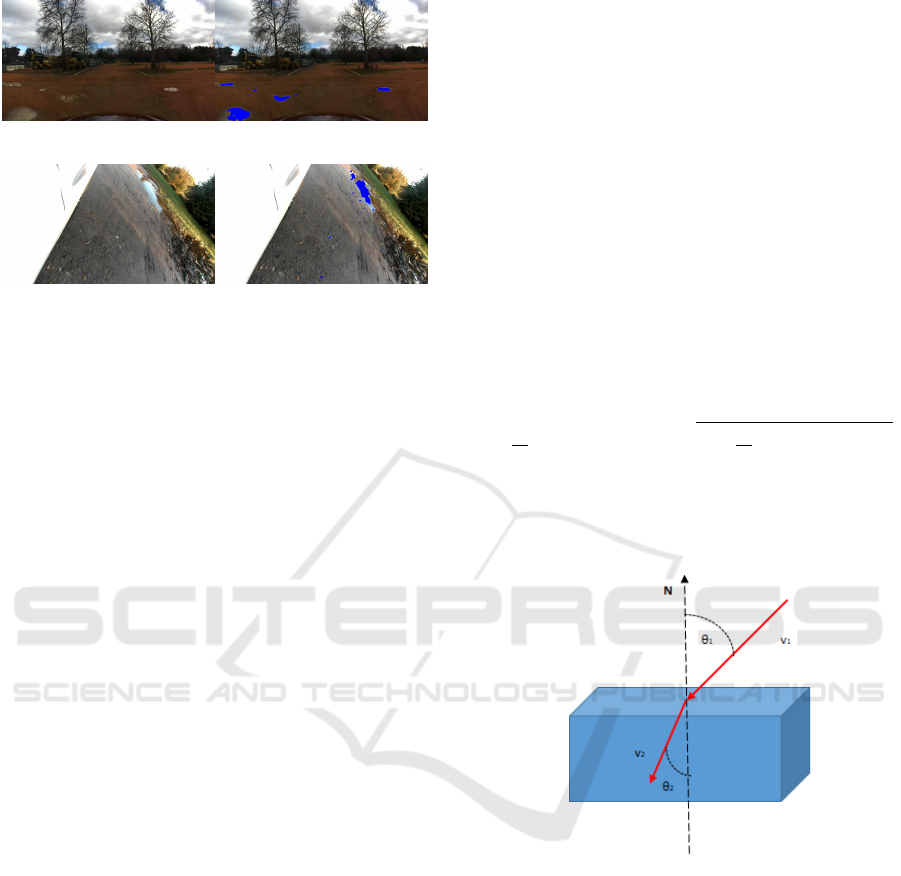
(a) Original frame (b) Segmented water hazards

(own)

Figure 2: Illustration of the DeepLab v3 (Chen et al.,

2018) network trained for water hazard segmentation on the

dataset of (Han et al., 2018) and own stereo camera data.

The segmented hazards are illustrated with blue color.

rises. However, with an appropriate camera installa-

tion, we can do both tasks with one camera. As 3D

environment reconstruction of the scene is continu-

ously made, it is enough to segment the water hazard

area only in one image to label the 3D scene for the

hazardous areas (alternatively water hazards can be

tracked through the scenes (Nguyen et al., 2017)),

3.2 Estimating Water Surface

To get a deterministic solution for the underwater

depth in the scale of the reconstruction of the sur-

roundings, we use the previously reconstructed point

cloud. We assume that the shore around the puddle

lies in the same plane as the water surface, or at least

it has the same normal, and the offset to the water sur-

face can be estimated from the reconstruction (tests

with artiﬁcial containers). Thus, in general, we esti-

mate the ground plane’s parameters with MSAC (Torr

and Zisserman, 2000), and we use the same param-

eters to describe the water surface. Alternatively, a

gyroscope can be used to determine the z direction

- the surface normal of the water - and knowing the

camera’s installation position can be enough to esti-

mate this plane’s offset. However, we propose to use

our proposed pipeline, as it is a more general solution

that can work in off-road scenarios with elevation and

angle differences in the path.

Our previous estimation of water hazard regions

can be made more precise with the ground model. As

triangulated points (without refraction correction) be-

low, this plane will correspond to the underwater sur-

face.

3.3 Calculating Underwater Depth

Our goal is to determine the underwater surface’s

true depth (using corresponding point pairs on the

images). Now, the camera positions and the water

surface are known. We can explicitly calculate the

X, Y , and Z coordinates of the previously matched

underwater points based on the following equations

(lens distortion effects have been already corrected).

Snell’s law is usually given in the scalar form :

· sinθ

= n

· sinθ

(1)

where n

and n

are the refraction indices of the

medium and θ

and θ

are the incidence and refrac-

tion angles.

Rewriting in vector form and rearranging it gives

for v

(the refraction vector) (Skarlatos and Agraﬁo-

tis, 2018):

[N × (−N × v

)] − N

1 −





(N × v

)(N ×v

)

(2)

where v

is the incidence vector, and N is the wa-

ter’s surface normal. The illustration can be seen in

Figure 3.

Figure 3: Illustration of Snell’s law.

Knowing the given camera’s intrinsic and extrin-

sic parameters, the projection matrix in a general co-

ordinate system can be written as:

C = I · T (3)

where I is the intrinsic matrix, and T is the 3x4 homo-

geneous transformation matrix transforming from the

global coordinate system to the camera coordinates.

The projection equation of a 3D point given by ho-

mogeneous global coordinates A = [X Y Z 1] to

an image point given by homogeneous image coordi-

nates a = [u v 1] can be rearranged to the form:

M · [X Y Z 1]

= 0 (4)

where the M matrix is:

Water Hazard Depth Estimation for Safe Navigation of Intelligent Vehicles



1,1

− uC

3,1

1,2

− uC

3,2

1,3

− uC

3,3

1,4

− uC

3,4

2,1

− vC

3,1

2,2

− vC

3,2

2,3

− vC

3,3

2,4

− vC

3,4



(5)

here C

i, j

are the elements of projection matrix in the

row and j

coloumn.

Equation 4 can be considered as equation of two

planes intersecting in a line which will be the ray of

projection through [u v] pixel coordinates. We can

determine the v

direction as the direction perpendic-

ular to the normal vectors of these planes (Figure 3).

= M

× M

(6)

where M

i = 1 : 2 indicates the ﬁrst three elements

of i

row of matrix M.

In the following, to triangulate the underwater

depth in case of a given point correspondence, two

camera poses are assumed. (The equations can be eas-

ily extended to more than two camera poses, and the

point coordinates can be determined by optimization

instead of triangulation.)

In case of two camera positions C

and C

the in-

tersection points of the water surface A

and A

(given

by coordinates X

, Y

, Z

, X

, Y

and Z

) with

two rays in direction of v

(ﬁrst camera) and v

(sec-

ond camera) can be determined by solving the equa-

tion system (Figure 4):

· X

+ N

·Y

+ N

· Z

= D (7)

= C

· v

(8)

where N

, N

and N

are the coordinates of the nor-

mal vector of the water surface and D is the scalar in

the plane equation of the surface, t

is the parameter

of the line equation, and i is the index of the given

camera pose.

After solving for A

and A

the underwater depth

can be triangulated by solving the following equation

system in a least-square sense for the point coordi-

nates P (Skarlatos and Agraﬁotis, 2018) (Figure 4):

· v

= A

· v

= P (9)

Note: We referred to (Skarlatos and Agraﬁotis,

2018) in case of two equations related to refraction

theory as they formalized these before us. However,

they do not use this in practice, as they utilized an em-

pirical formula to calculate a corrected focal length

for the water and do the correction on images (instead

of 3D coordinates). Their work is hardly comparable

to ours as they propose to use commercial software

and orthophotos for an entirely different purpose, cre-

ating digital surface models (DSM).

4 REAL-LIFE EXPERIMENTS

We have executed several experiments in different en-

vironments. We differentiate three types of tests we

have made, quantitative measurements with artiﬁcial

and natural water reservoirs with a mono camera, and

qualitative measurements with a stereo camera rig in-

stalled on a car.

In the following, the quantitative mono camera

(more complex computation) tests are presented. In

artiﬁcial reservoirs (e.g., pool), the underwater ge-

ometry is known or manually measured. Natural

reservoirs like puddles, water hazards in roads, and

brooklets were reconstructed (Figure 5). To generate

ground truth data in a natural reservoir, we created the

SfM model of the environment without the water in it,

manually registered the two point clouds, and the er-

ror is measured as the distance from each estimated

underwater points to the meshed surface. We gener-

ated ground truth data in this way for three scenes.

They were used in our quantitative evaluation.

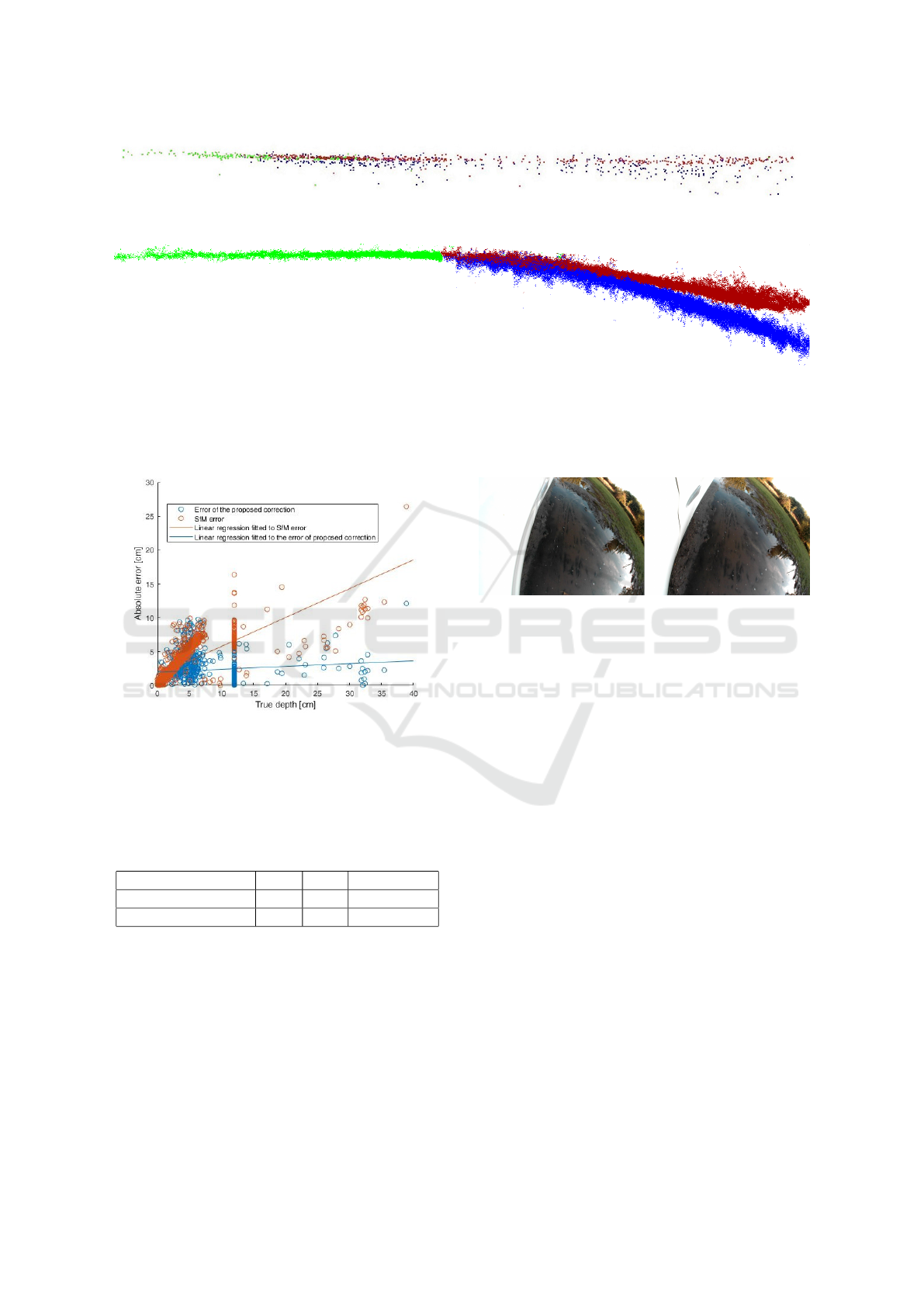
Quantitative results of the proposed depth correc-

tion are illustrated in Figure 7, where we approxi-

mated with a linear regression of the error of the SfM

depth estimation and our one. The approximation is

based on about 3000 points from different scenes; on

average, about 7 frames were used for reconstruction.

If a point was visible from more than one view, we

averaged the triangulations and ﬁltered the obviously

wrongly triangulated points above the water level. As

shown in the ﬁgure, in our evaluation there were nu-

merous points in the underwater depth range between

10 and 40 cm, but most of the points are below 10

cm (puddles). We neglected the number of measured

points deeper than 40 cm in the ﬁgure for better illus-

tration, as there were very few of them (they are ap-

proximately on the regression line) and also it is not

realistic to meet such deep potholes. As it is visible in

the ﬁgure, with our proposed correction, the error can

be approximated almost as a constant. The error of

SfM approximation is increasing with the depth. This

phenomenon is explained by Eq. 11 (in Section 5.2)

as it shows in the case of one viewpoint and a given

incidence angle, the apparent depth is linearly depen-

dent on the real one (with our correction, only other

errors of the process remain).

The mean absolute error in our tests with the pro-

posed correction was 2.15 cm, which is affected by

the triangulation error and by the accuracy of the

ground truth model (in the case of natural reservoirs).

That is why we did a separate evaluation for the cases

of artiﬁcial and natural reservoirs. Table 1 shows that

using our proposed correction pipeline gives a signiﬁ-

cant improvement compared to the SfM baseline. Our

VEHITS 2021 - 7th International Conference on Vehicle Technology and Intelligent Transport Systems

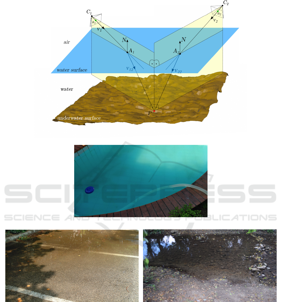
Figure 4: Illustration of underwater depth calculation of a P point seen by two cameras.

(a) Pool

(b) Water hazard (c) Brooklet

Figure 5: Example images used in reconstruction of different test scenes.

goal is to estimate the depth of natural ones. How-

ever, error estimation is more straightforward in the

case of geometric surfaces (artiﬁcial reservoirs). Be-

sides, examining the artiﬁcial reservoirs allowed us to

investigate the proposed correction in deeper water.

The errors of the proposed pipeline are compara-

ble to the one reported in (Dietrich, 2017). The author

of it also tested in artiﬁcial (pool with 0.32 cm mean

absolute error) and natural water reservoirs (5.6 cm

and 3.9 cm mean absolute error - in different time pe-

riods). It should be noted that the authors used georef-

erenced orthophotography (getting a more precise ini-

tial point cloud) and less a general solution to achieve

those results.

Figure 6 shows a qualitative illustration of the pro-

posed method. Using only SfM to reconstruct under-

Water Hazard Depth Estimation for Safe Navigation of Intelligent Vehicles

(a) Mono camera

(b) Stereo camera pair

Figure 6: Example point clouds (from different scenes) generated about underwater surface with and without correction.

Green points indicates the ground surface, red ones are the points without the proposed correction and blue ones are the ones

with the correction.

Figure 7: Linear regression to the errors of different ap-

proximation of underwater depth. Note: Vertical line corre-

sponds to artiﬁcial reservoir with ﬂat underwater surface.

Table 1: Absolute error in different test scenarios [cm]. SfM

refers to standard Structure from Motion with COLMAP

(Sch

onberger and Frahm, 2016) (Sch

onberger et al., 2016),

[1] refers to (Dietrich, 2017) (on their own scenes) and

’Correction’ refers to our proposed correction method.

Depth calculation SfM [1] Correction

Artiﬁcial reservoirs 6.55 0.32 1.55

Natural reservoirs 2.60 3.9 2.26

water points (red points) resulted in an approximately

ﬂat surface at approximately ground (black points)

level. However, with the proposed correction (blue

points), the real underwater surface can be seen. (In-

creasing depth is visible.) A similar phenomenon can

be observed in a point cloud acquired by a stereo cam-

era rig.

In the stereo camera case, as the traversing of the

exact routes was nearly impossible, ground truth data

were not recorded. Instead of that, we will use these

Figure 8: Example image for off-road depth estimation

from our stereo camera dataset.

data to prove our method can be applied in a real-

time driving application. We gathered about half an

hour recording, where about 14 % of the frames con-

tained water hazards. Processing the image pairs of

resolution 1520x1080 requires about 290 ms from

which our depth estimation takes 60 ms in a com-

puter of Intel Core i7-4790K @4.00GHz processor,

32 GB RAM and nVidia GTX 1080 graphic card with

Windows 10 operating system in Matlab environment.

This means that the process can run in this conﬁgura-

tion about 4 frame per second. We illustrate (qualita-

tively) our method on the recorded stereo data (Figure

2, 7 and 8) as well.

5 DISCUSSION

In this section we provide some discussion about the

proposed method.

5.1 Implementation Issues

The 4 FPS process speed is already satisfying as depth

estimation is not necessary for every frames (only de-

tection so that the vehicle can start deceleration from

a sufﬁcient distance).

VEHITS 2021 - 7th International Conference on Vehicle Technology and Intelligent Transport Systems

Assuming a 1.5 m height and 30 degrees tilted

camera installation (ﬂat ground) at the optical centre

of the camera we will get a 60 degree incidence an-

gle. This means about 2.6 m distance on the ground

to the water hazard. Considering the process speed

(and constant velocity) the vehicle must slow down to

9 m/s ( 32 km/h) before reaching this distance. As

the hazards can be detected a lot more farther this is

not extraordinary in an off-road or (pothole ﬁlled) on-

road environment for safe navigation.

Optimized implementation e.g. in C++ environ-

ment can speed up even more the estimation, also de-

creasing the image resolution or number of points to

which underwater depth is estimated also reduces the

execution time to a large extent. (In our experience

SfM provides fewer points by two order of magnitude

than stereo, but they also provide meaningful depth

result.)

5.2 Signiﬁcance of Depth Correction

In the stereo camera case, as the cameras are very

close to each other (we used Omnivision OV4689

CMOS sensor with about 5.8 cm baseline in our case)

and the water surface is relatively far (at least 1 m,

based on camera installation on the vehicle), the inci-

dence angle is approximately the same. So, the one

viewpoint model is a good approximation (in general

SfM case, there can be very different incidence angles

and camera positions).

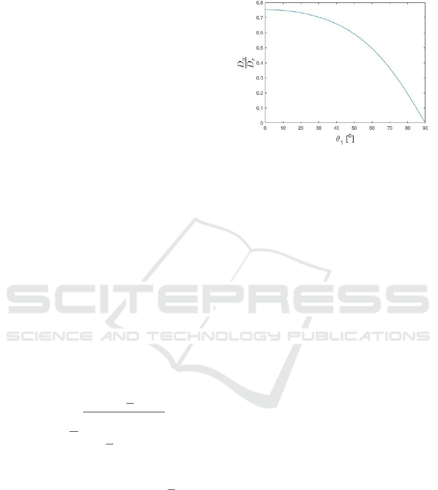
We can write the equality with the the apparent

depth (D

) and the real (D

) one:

· tan θ

= D

· tan θ

(10)

From that, we get:

= D

tan(arcsin(

sinθ

))

tanθ

(11)

The resulted

ratio is plotted in Figure 9 be-

tween 0 and 90 degrees for

= 0.75 (water n

= 1.33

and air n

= 1.0 refraction indices, considered as con-

stant in this paper). As one can see, at least about 25

% error is produced without any correction (coming

from the value of the initial depth ratio is

). How-

ever, 0 degree incidence angle (perpendicular to the

water surface) is not practical in a driving application

(as mentioned before). As the incidence angle goes

to 90 degrees, the refraction angle goes to the critical

angle, and the ratio of apparent and real depth goes

to 0, meaning that we can estimate 0 depth (ground

level) no matter how deep in reality the hazard is (in

theory, in practice the maximum of θ

is about 60 de-

grees, as we said earlier). That is why the correction

of the paper is very important.

Figure 9: Ratio of apparent and real depth.

5.3 Comparison

There are papers referred in our work (Section 2 §5)

which deal with underwater depth correction for com-

pletely different purpose and circumstances. We com-

pared our method to one of them in Table 1. However,

it is very important to note:

The depth correction problem of our scenes (images

from general viewpoints) cannot be solved by the

methods referred in this paper in Section 2 (or any

other previous depth correction method to the best of

our knowledge).

Also, as our depth correction problem is the general

solution of those papers simpliﬁcations’ (we estimate

parameters assumed to be known by others). That is

why, there is no point in further comparison to the

scene of earlier works. As knowing the parameters

they need for their calculation, we would get the same

simpliﬁed equations they use (instead of the ones we

apply), and so the same results as they.

5.4 Other Application Areas

We designed our method to apply it in case of au-

tomation of ground vehicles in an off-road or on-road

(with potholes) environment. However, other vehi-

cles, intelligent systems can proﬁt from the proposed

method as well. For example, UAV exploration of the

terrain also can utilize our underwater surface estima-

tion. For bathymetric mapping purposes or search and

rescue missions in case of a ﬂood. (In the latter case,

the water level should be known to assess the degree

of risk and choose the right vehicle for the rescue.)

(Gomez and Purdie, 2016)

Water Hazard Depth Estimation for Safe Navigation of Intelligent Vehicles

6 CONCLUSIONS

In this paper, we presented a novel approach to re-

construct an underwater surface with a mono cam-

era. The method does not require any restriction of

the camera motion or speciﬁc sensors, and the 3D co-

ordinates of underwater surface points can be deter-

mined in a least-square sense. The method is useful

to increase vehicles’ intelligence with water hazard

depth estimation both in on-road and off-road cases.

This phenomenon was illustrated in real-life scenar-

ios with onboard stereo cameras.

The method will be more elaborated for practical so-

lutions, as we would like to investigate how other ve-

hicles, transportation system can beneﬁt from our pro-

posed method, and what is the optimal optical struc-

ture for the different vehicles.

ACKNOWLEDGEMENTS

The research presented in this paper, carried out by

Institute for Computer Science and Control was sup-

ported by the Ministry for Innovation and Technology

and the National Research, Development and Innova-

tion Ofﬁce within the framework of the National Lab

for Autonomous Systems.

REFERENCES

Agraﬁotis, P., Karantzalos, K., Georgopoulos, A., and Skar-

latos, D. (2020). Correcting image refraction: To-

wards accurate aerial image-based bathymetry map-

ping in shallow waters. Remote Sensing, 12(2).

Agraﬁotis, P., Skarlatos, D., Georgopoulos, A., and

Karantzalos, K. (2019). Shallow water bathymetry

mapping from uav imagery based on machine learn-

ing. ISPRS - International Archives of the Photogram-

metry, Remote Sensing and Spatial Information Sci-

ences, XLII-2/W10:9–16.

Agrawal, A., Ramalingam, S., Taguchi, Y., and Chari, V.

(2012). A theory of multi-layer ﬂat refractive geom-

etry. In 2012 IEEE Conference on Computer Vision

and Pattern Recognition, pages 3346–3353.

Chari, V. and Sturm, P. (2009). Multi-view geometry of the

refractive plane.

Chen, L., Yang, J., and Kong, H. (2017). Lidar-histogram

for fast road and obstacle detection. In 2017 IEEE

International Conference on Robotics and Automation

(ICRA), pages 1343–1348.

Chen, L.-C., Zhu, Y., Papandreou, G., Schroff, F., and

Adam, H. (2018). Encoder-decoder with atrous sep-

arable convolution for semantic image segmentation.

In Proceedings of the European Conference on Com-

puter Vision (ECCV).

Costa, B., Battista, T., and Pittman, S. (2009). Com-

parative evaluation of airborne lidar and ship-based

multibeam sonar bathymetry and intensity for map-

ping coral reef ecosystems. Remote Sensing of Envi-

ronment, 113(5):1082 – 1100.

Dietrich, J. T. (2017). Bathymetric structure-from-motion:

extracting shallow stream bathymetry from multi-

view stereo photogrammetry. Earth Surface Processes

and Landforms, 42(2):355–364.

Fryer, J. (1983). Photogrammetry through shallow water.

Australian journal of geodesy, photogrammetry, and

surveying, 38:25–38.

Fryer, J. G. and Kniest, H. T. (1985). Errors in depth

determination caused by waves in through-water

photogrammetry. The Photogrammetric Record,

11(66):745–753.

Gomez, C. and Purdie, H. (2016). UAV- based photogram-

metry and geocomputing for hazards and disaster risk

monitoring – a review. Geoenvironmental Disasters,

Han, X., Nguyen, C., You, S., and Lu, J. (2018). Single

image water hazard detection using FCN with reﬂec-

tion attention units. In Proceedings of the European

Conference on Computer Vision (ECCV).

Haris, M. and Hou, J. (2020). Obstacle detection and safely

navigate the autonomous vehicle from unexpected ob-

stacles on the driving lane. Sensors, 20:4719.

Heikkila, J. and Silven, O. (1997). A four-step camera cal-

ibration procedure with implicit image correction. In

Proceedings of IEEE Computer Society Conference

on Computer Vision and Pattern Recognition, pages

1106–1112.

Hirschmuller, H. (2005). Accurate and efﬁcient stereo pro-

cessing by semi-global matching and mutual informa-

tion. In 2005 IEEE Computer Society Conference on

Computer Vision and Pattern Recognition (CVPR’05),

volume 2, pages 807–814 vol. 2.

Jordt-Sedlazeck, A. and Koch, R. (2013). Refractive

structure-from-motion on underwater images. In 2013

IEEE International Conference on Computer Vision,

pages 57–64.

Kang, L., Wu, L., and Yang, Y.-H. (2012). Two-view un-

derwater structure and motion for cameras under ﬂat

refractive interfaces. In Fitzgibbon, A., Lazebnik, S.,

Perona, P., Sato, Y., and Schmid, C., editors, Com-

puter Vision – ECCV 2012, pages 303–316, Berlin,

Heidelberg. Springer Berlin Heidelberg.

Maas, H.-G. (2015). On the accuracy potential in under-

water/multimedia photogrammetry. Sensors (Basel,

Switzerland), 15:18140–52.

Mettes, P., Tan, R. T., and Veltkamp, R. C. (2017). Water de-

tection through spatio-temporal invariant descriptors.

Computer Vision and Image Understanding, 154:182

– 191.

Murai, S., Kuo, M.-Y. J., Kawahara, R., Nobuhara, S., and

Nishino, K. (2019). Surface normals and shape from

water. In Proceedings of the IEEE/CVF International

Conference on Computer Vision (ICCV).

Mustaniemi, J., Kannala, J., S

arkk

a, S., Matas, J., and

Heikkil

a, J. (2017). Inertial-based scale estimation

VEHITS 2021 - 7th International Conference on Vehicle Technology and Intelligent Transport Systems

for structure from motion on mobile devices. In

2017 IEEE/RSJ International Conference on Intelli-

gent Robots and Systems (IROS), pages 4394–4401.

Nguyen, C. V., Milford, M., and Mahony, R. (2017). 3D

tracking of water hazards with polarized stereo cam-

eras. In 2017 IEEE International Conference on

Robotics and Automation (ICRA), pages 5251–5257.

Qian, Y., Zheng, Y., Gong, M., and Yang, Y.-H. (2018). Si-

multaneous 3D reconstruction for water surface and

underwater scene. In Proceedings of the European

Conference on Computer Vision (ECCV).

Qiao, J. J., Wu, X., He, J. Y., Li, W., and Peng, Q. (2020).

Swnet: A deep learning based approach for splashed

water detection on road. IEEE Transactions on Intel-

ligent Transportation Systems, pages 1–14.

Rankin, A. and Matthies, L. (2010). Daytime water detec-

tion based on color variation. In 2010 IEEE/RSJ In-

ternational Conference on Intelligent Robots and Sys-

tems, pages 215–221.

Sch

onberger, J. L. and Frahm, J.-M. (2016). Structure-

from-motion revisited. In Conference on Computer

Vision and Pattern Recognition (CVPR).

Sch

onberger, J. L., Zheng, E., Pollefeys, M., and Frahm, J.-

M. (2016). Pixelwise view selection for unstructured

multi-view stereo. In European Conference on Com-

puter Vision (ECCV).

Shan, J. (1994). Relative orientation for two-media

photogrammetry. The Photogrammetric Record,

14(84):993–999.

Skarlatos, D. and Agraﬁotis, P. (2018). A novel iterative

water refraction correction algorithm for use in struc-

ture from motion photogrammetric pipeline. Journal

of Marine Science and Engineering, 6(3).

Song., R., Wetherall., J., Maskell., S., and Ralph., J. F.

(2020). Weather effects on obstacle detection for au-

tonomous car. In Proceedings of the 6th Interna-

tional Conference on Vehicle Technology and Intelli-

gent Transport Systems - Volume 1: VEHITS,, pages

331–341. INSTICC, SciTePress.

Terwisscha van Scheltinga, R. C., Coco, G., Kleinhans,

M. G., and Friedrich, H. (2020). Observations of dune

interactions from dems using through-water structure

from motion. Geomorphology, 359:107126.

Torr, P. H. S. and Zisserman, A. (2000). MLESAC: A new

robust estimator with application to estimating image

geometry. Computer Vision and Image Understand-

ing, 78:138–156.

Xie, B., Pan, H., Xiang, Z., and Liu, J. (2007). Polarization-

based water hazards detection for autonomous off-

road navigation. In 2007 International Conference on

Mechatronics and Automation, pages 1666–1670.

Zhang, Z. (2000). A ﬂexible new technique for camera cal-

ibration. IEEE Transactions on Pattern Analysis and

Machine Intelligence, 22(11):1330–1334.

Zhao, Y., Li, J., Guo, L., Deng, Y., and Raymond, C. (2014).

Water hazard detection for intelligent vehicle based on

vision information. Recent Patents on Computer Sci-

ence, 7.

Water Hazard Depth Estimation for Safe Navigation of Intelligent Vehicles