Research on Optimization of 4G-LTE Wireless Network Cells Anomaly

Diagnosis Algorithm based on Multidimensional Time Series Data

Bing Qian

, Chong Ma

1 a

and Tong Zhang

Beijing Research Institute, China Telecom Corporation Limited, Beijing, China

Intel Corporation, Santa Clara, California, U.S.A.

Keywords:

Multidimensional Time Series Data, Anomaly Detection, Unsupervised Learning.

Abstract:

With the continuous increase of network terminal equipment, the operation scenarios of 4G-LTE wireless

networks are becoming more and more complex. The traditional manual method of analysis and screen-

ing of network cell equipment can no longer meet the needs of production. Therefore, an efﬁcient wireless

network cell abnormality diagnosis algorithm is needed to screen abnormalities of equipment to improve op-

eration and maintenance efﬁciency. In view of the fact that the existing single-dimensional anomaly diagnosis

algorithm cannot achieve fully automated detection and the existing multidimensional anomaly diagnosis al-

gorithm has low detection efﬁciency on multidimensional time series data, there are a large number of errors

and omissions. This paper proposes a multidimensional time series data based on 4G-LTE wireless network

cell anomaly diagnosis optimization algorithm uses small-sample supervised algorithms to assist the training

of massive-sample unsupervised algorithms, thereby improving the detection performance of unsupervised

learning algorithms. This paper veriﬁes the effectiveness of the optimization algorithm through experiments,

and has a great improvement in the four commonly used unsupervised algorithms, which can well improve the

anomaly detection capabilities of the existing algorithms.

1 INTRODUCTION

With the continuous development of communication

technology, the layout of wireless networks has be-

come more complex, and the operation and main-

tenance of network equipment has become more

and more challenging. The number of existing 4G-

LTE base stations is huge and there are many prob-

lems. However, the limited maintenance resources,

the shortage of personnel, and the lack of support

methods and platforms make it difﬁcult to achieve in-

depth and detailed maintenance. How to reduce the

impact of faults on the business and improve user ex-

perience under the existing circumstances is the top

priority of maintenance work. At present, the tra-

ditional operation and maintenance method of wire-

less base stations is to monitor equipment alarms and

network indicators by engineers, identify abnormal

points, and manually analyze, screen, locate, and pro-

cess. The efﬁciency of manual screening is low, and

the skill level of maintenance personnel is uneven, re-

sulting in an inability to effectively improve mainte-

https://orcid.org/0000-0001-8602-4676

nance efﬁciency. Therefore, in order to realize fault

detection automation and reduce manual participa-

tion, it is necessary to develop a detection algorithm

for wireless network cell abnormality.

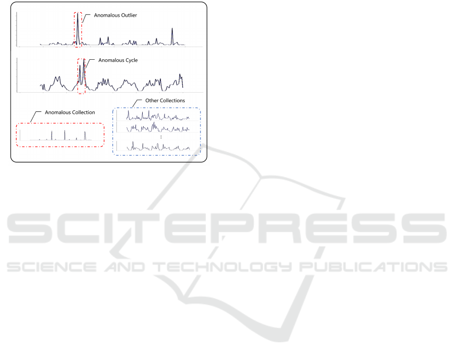
The anomalies of wireless network cell can be

classiﬁed into three categories: anomalous outliers,

anomalous cycles, and anomalous collections (Chan-

dola et al., 2009). As shown in Figure 1, in aperi-

odic data, if a single data point can be considered

anomalous relative to other data, the data is called

an outlier. In a periodic sequence, if the data is ab-

normal in a certain period but normal in other pe-

riods, the data is called abnormal period data. In

time series collections, if the collection where the data

is located is inconsistent with other sibling collec-

tions, the collection is an abnormal collection. This

paper performs anomaly detection on wireless net-

work cell devices. The above three anomalies need

to be included. For a 4G-LTE wireless network cell,

the device reports monitoring data every hour. The

monitoring data contains multiple indicators, includ-

ing PDCP (Packet Data Convergence Protocol) layer

data ﬂow, RRC (Radio Resource Control) connec-

tion times, CQI (Channel Quality Indicator) excellent

Qian, B., Ma, C. and Zhang, T.

Research on Optimization of 4G-LTE Wireless Network Cells Anomaly Diagnosis Algorithm based on Multidimensional Time Series Data.

DOI: 10.5220/0010434000480057

In Proceedings of the 6th International Conference on Internet of Things, Big Data and Security (IoTBDS 2021), pages 48-57

ISBN: 978-989-758-504-3

rate, and so on. Within a week’s time sequence win-

dow, the point abnormality and periodic abnormality

of each indicator at a certain moment will affect the

failure judgment of a single network cell. At the same

time, different sets of network cells need to be com-

pared to detect anomalies that are different from other

sibling network cell collections.

Figure 1: Three kinds of 4G-LTE wireless network cell

anomalies: anomalous outliers, anomalous cycles, and

anomalous collections.

2 RELATED WORK

In wireless network cell anomaly detection, the exist-

ing single-dimensional anomaly diagnosis algorithm,

whether it is traditional machine learning such logis-

tic regression (Kleinbaum et al., 2002) or deep learn-

ing algorithms such TCN (Bai et al., 2018), these

algorithms ﬁrstly predict the index value at the fu-

ture moment, then set the threshold of the difference

between the predicted data and the real data to de-

cide whether it is abnormal. This method has some

limitations. On the one hand, it can only judge the

abnormal value of a single indicator. To determine

whether the network cell is abnormal according to the

single indicator, it also needs to rely on the voting

between the indicators or other manually formulated

combination rules. On the other hand, this method

can only detect point anomalies and partial periodic

anomalies, and cannot compare the wireless network

cell data set with other sibling sets. Therefore, the

single indicator anomaly detection algorithm is not

suitable for the scenario in this paper. This paper

needs to be modeled by combining statistical fea-

ture extraction and multidimensional anomaly diag-

nosis algorithm. Statistical feature extraction mainly

includes the construction of time series features and

set features. Multidimensional anomaly diagnosis al-

gorithms include supervised algorithms with labeled

data, such as SVM(George and Vidyapeetham, 2012),

ANN(Pradhan et al., 2012), and unsupervised algo-

rithms with unlabeled data, such as k-Means(Wazid

and Das, 2016). Generally, the results of supervised

algorithms are more reliable and accurate than unsu-

pervised algorithms. However, due to the amount of

abnormal data is much less than normal data, a larger

amount of data is required to train an effective su-

pervision model, which means that it will cost a lot

to label the data. Therefore, supervised anomaly de-

tection algorithms are actually not suitable for large-

scale multi-dimensional anomaly detection Scenes.

Although unsupervised anomaly detection algorithms

do not require labeling data and are more suitable for

massive data scenarios, multidimensional unsuper-

vised algorithms cannot select useful features, these

mixed useless features will reduce the accuracy of

unsupervised models. This paper designs a method

of coupling supervised and unsupervised algorithms

for training. We have obtained a small number of

4G-LTE wireless network cell annotation data. These

data come from multiple operation and maintenance

engineers, but we found that different operation and

maintenance engineers have different understandings

of the same data. They rely on their own operation

and maintenance experience, and it is difﬁcult to unify

their opinions. Therefore, we believe that these an-

notation data not only contain reliable abnormal la-

bels, but may also contain noisy normal data (False

alarms), which is a low-quality annotation data. If a

model with high accuracy is obtained through super-

vised algorithm training with this data, then its gener-

alization performance on a large number of samples

is not excellent. We ﬁrst analyze these low-quality

annotation data to ﬁnd useful features, and then use

these useful features to train unsupervised algorithms.

The anomaly detection ability of the unsupervised

model is improved through the coupling training of

the unsupervised algorithm and the supervised algo-

rithm.

General anomaly diagnosis algorithms such as

anomaly detection based on measure density and

KNN (Angiulli and Pizzuti, 2002), Auto Encoder

based on neural network (Aggarwal, 2015), anomaly

detection based on projected distance and PCA (Shyu

et al., 2003), Isolation Forest (Aryal et al., 2014),

One Class SVM (Wang et al., 2004), KDE (Kim

and Scott, 2012), etc., cannot simultaneously ﬁnd

abnormal outliers, abnormal cycles, and abnormal

collections. After comparing various algorithms,

we selected the four algorithms with the best ef-

fects for analysis and subsequent experiments. As

shown in Figure 2, it can be seen that KNN and

Research on Optimization of 4G-LTE Wireless Network Cells Anomaly Diagnosis Algorithm based on Multidimensional Time Series Data

Figure 2: Abnormal state that could not be fully detected.

Each curve represents the change in the value of a single

indicator of the network cell within a week. Figure (a) rep-

resents the abnormal detection of the E-RAB Abnormal in-

dicator of the network cell using the anomaly detection al-

gorithm based on measurement density and KNN. The ab-

scissa is the time point, the ordinate is the indicator value.

The red legend represents the detected abnormal curve.

Blue represents the detected normal curve. Yellow repre-

sents a curve that the algorithm detects as normal but is ac-

tually abnormal. Figure (b) represents the detection result

of the E-RAB Abnormal indicator by the One Class SVM

algorithm. Figure (c) represents the detection result of the

RRC AttConnReestab indicator by the Isolation Forest al-

gorithm. Figure (d) represents the detection result of the

PCA algorithm on the RRC AttConnReestab indicator.

One Class SVM cannot perfectly detect wireless net-

work cells different from other collections, such as

E-RAB AbnormRel (Evolved Radio Access Bearer

Abnormally Released) anomaly. Isolation Forest and

PCA also have the problem of missed detection of

RRC AttConnReestab (Radio Resource Control At-

tach Connection Reestablish) anomaly. These unsu-

pervised algorithms are often unable to ﬁnd out the

anomalies in this scenario comprehensively. There-

fore, based on the existing small number of expert

system annotated samples and massive non-annotated

samples, this paper designs a training method that

combines supervised and unsupervised algorithms,

which can improve the detection performance of un-

supervised algorithms.

3 METHODOLOGY

We ﬁrst deﬁned 3 anomaly types for the time series

data of 4G-LTE wireless network cells, and then we

proposed a method to train an unsupervised anomaly

diagnosis algorithm assisted by a supervised model.

3.1 Problem Deﬁnition

In this paper, all the time series window data is shown

in Figure 3, which can be regarded as the set X, the

single network cell time series window is the set X

the relationship between the two can be expressed as

X = X

, X

, ..., X

, n represents the number of network

cells included in set X. The multidimensional data

at a single moment in the time series window is S

= S

, S

, ..., S

, t is the time series length, and the

multidimensional data S

= s

, s

, ..., s

, k represents

the indicator dimension.

Figure 3: Time series window data.

The problem to be solved in this paper is

that in the data set X containing many network

cells, an abnormal network cell X

is detected by

a multidimensional unsupervised algorithm. The

basis for judging the abnormality of the network

cell X

is that an indicator sequence S

, S

, ..., S

,l ∈ (1, ..., k) in X

has an anomalous outlier S

abnormal

(anomalous outliers) or an abnormal sub-sequence

, S

(

a + 1)

, ..., S

(

a +t)

, a ∈ (1, ...c

(

n −t)) (anoma-

lous cycles), or the sequence (anomalous collection)

is inconsistent with the indicator sequence changes of

other network cells. Synthesize abnormal outlier, ab-

normal cycle detection and abnormal detection of net-

work cell collections to determine abnormal network

cell.

3.2 Our Method

This paper mainly assists the unsupervised algorithm

to select important features through a supervised algo-

rithm, and improves the performance of the unsuper-

vised anomaly detection algorithm. As shown in Fig-

ure 4, in the 4G-LTE wireless network cell anomaly

detection scenario, ﬁrst, the features of the original

data are constructed based on the statistical method to

form the original feature data set, and the data is pre-

processed. And then divided into annotated set and

non-annotated set according to whether it has been

labeled. Then use supervised algorithms such as XG-

Boost (Chen and Guestrin, 2016) to train the anno-

tated set and calculate the feature importance, select

IoTBDS 2021 - 6th International Conference on Internet of Things, Big Data and Security

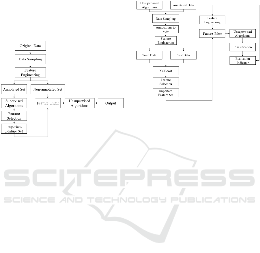
the important feature set by sorting the important fea-

tures (Chen et al., 2019), and ﬁlter the non-annotated

data features, and ﬁnally use KNN, PCA, Isolation

Forest, One Class SVM and other unsupervised al-

gorithms are trained on non-annotated sets to obtain

classiﬁcation results.

Figure 4: Our anomaly detection algorithm process.

Because the non-annotated data cannot be veri-

ﬁed, it is only used in the real reasoning stage. As

shown in Figure 5, in order to verify the effective-

ness of the algorithm in this paper, we conduct exper-

iments on the annotated data. First, 4 unsupervised

algorithms (KNN, PCA, Isolation Forest, One Class

SVM) are used to calculate the anomaly labels, and

then vote together with the labels marked by experts.

The rule is that if 3 of the 5 tags are marked as abnor-

mal, the data is counted as an abnormal point, other-

wise it is a normal point. Then construct features on

the voting data through feature engineering, divide the

training data and test data, and then train the XGBoost

model, sort the importance of the features constructed

by the feature engineering according to the XGBoost

algorithm, and intercept the ﬁrst 100 features as im-

portant feature sets. Then ﬁlter the features of the

original annotation data, respectively train 4 unsuper-

vised algorithms, and calculate the evaluation indica-

tor according to the predicted label and ground truth.

Finally, the effectiveness of the algorithm is veriﬁed

by comparing the evaluation indicator of four unsu-

pervised algorithms before and after feature selection.

4 DATA PREPROCESSING

In this paper, the original data is ﬁrst screened, some

data with more missing time series are removed.

Then, some of the original indicators with higher

correlation coefﬁcients are deleted, because indica-

Figure 5: The process of validating the algorithm.

tors with higher correlations have lower discrimina-

tion and will affect the training of the linear model.

Next, construct statistical features and time series fea-

tures of the remaining indicators through feature en-

gineering. Finally, since what we obtained is a kind of

low-quality and unreliable annotation data, in order to

enhance the credibility of the annotation data, we use

the unsupervised anomaly detection algorithm and the

expert mark to perform majority voting to determine

the anomaly label.

4.1 Data Sampling

Data Scenes Screening. The original data contains

a total of 6 scenes of data, including high-speed rail,

colleges, residential buildings, subways, etc. This pa-

per selects the wireless network cell data of the res-

idential scene. Because the data of the residential

scene has a high proportion, and the data of the res-

idential scene has a certain periodicity in time, it is

convenient for experiment and analysis.

Data Cleaning. The data set of each wireless net-

work cell should contain 7 × 24 hours of time series

data, but in the actual data collection process, there

are some data reports that are repeated or lost. This

paper ﬁrst removes the data with the same wireless

network cell id and the same timestamp, then, the col-

lection with less than 3% of missing cells is screened,

and ﬁnally the number of wireless network cell col-

lections is 4188, and the hourly granularity data is

688747.

4.2 Feature Engineering

Original Indicators. The original indicators are

shown in Table 1, which contains 24 kinds of indi-

cators.

Research on Optimization of 4G-LTE Wireless Network Cells Anomaly Diagnosis Algorithm based on Multidimensional Time Series Data

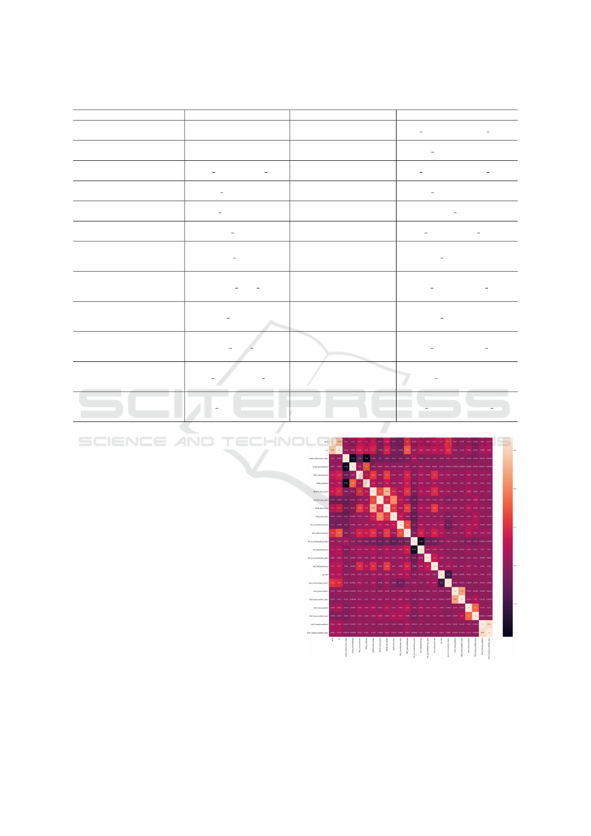
Table 1: Original indicators.

Meaning Name Meaning Name

PDCP trafﬁc pdcp

Same frequency switching

success rate

HO SuccOutIntraFreq Rate

RRC connection times rrc

Number of failed same

frequency switching

HO FailOutIntraFreq

Radio initial connection

success rate

Radio InitSuccConn Rate

Inter-frequency switching

success rate

HO SuccOutInterFreq Rate

S1 signaling connection

establishment failure times

S1Sig FailConnEstab

Number of failed inter-

frequency switching

HO FailOutInterFreq

RRC connection establish-

ment failure times

RRC FailConnEstab CQI excellent rate cqi rate

E-RAB establishment

failure times

ERAB FailEstab

PRB average interference

noise

phy rrurxrssimean chan1

Number of abnormal

releases of UE context

UECNTX AbnormRel

Packet loss number of

uplink user interface

of air port

PDCP SduLossPktUl

UE context drop rate UECNTX Drop Rate

Packet loss rate of

uplink user interface

of air port

PDCP SduLossPktUl Rate

E-RAB abnormal

release times

ERAB AbnormRel

Packet loss number of

downlink user interface

of air port

PDCP SduLossPktDl

E-RAB drop rate ERAB Drop Rate

Packet loss rate of

downlink user interface

of air port

PDCP SduLossPktDl Rate

RRC connection reestablish

rate

RRC ConnReestab Rate

Packet discard number

of downlink user interface

of air port

PDCP SduDiscardPktDl

RRC reconstruction

request times

RRC AttConnReestab

Packet discard rate of

downlink user interface

of air port

PDCP SduDiscardPktDl Rate

Correlation Analysis. Calculate the Pearson corre-

lation (Lee Rodgers and Nicewander, 1988) between

the original indicators two by two. The results are

shown in Figure 6. The original indicators with corre-

lation coefﬁcient > 0.7 are selected and deleted. The

deleted indicators are shown in Table 2.

Generate Features. Construct features from the 21

original indicators retained through feature engineer-

ing. This paper constructs 3 feature sets, namely sta-

tistical feature set, time feature set, and time series

feature set. The statistical feature set calculates the

maximum, minimum, mean, standard deviation, and

median on the time series for a single indicator of each

wireless network cell; the time feature set includes

the hour corresponding to the time stamp and the day

of the week, whether it is a weekend, whether it is a

holiday; time series feature set include the maximum,

minimum, mean, standard deviation, and median of a

single indicator at the same hour in a week, and the

value of a single indicator in the previous hour. The

generated feature set is shown in Table 3.

Generate Labels. After the data is constructed

through feature engineering, 4 unsupervised algo-

rithms KNN, PCA, Isolation Forest, and One Class

SVM are trained separately, and the prior anomaly ra-

Figure 6: Correlation between original indicators.

tios of the four algorithms are set to 1%, calculate the

abnormal label through unsupervised algorithm, and

IoTBDS 2021 - 6th International Conference on Internet of Things, Big Data and Security

Table 2: Delete the original indicator.

Indicator 1 Status Indicator 2 Status Correlation

pdcp Keep rrc Delete 0.83

PDCP SduDiscardPktDl Keep PDCP SduDiscardPktDl Rate Delete 0.74

PDCP SduLossPktUl Keep PDCP SduLossPktUl Rate Delete 0.94

Table 3: Constructing features based on original indicators.

Feature set Meaning Name

Input

(dim)

Output

(dim)

Statistical

Features

The maximum value of a single indicator in time series kpi max

21 105

The minimum value of a single indicator in time series kpi min

The mean value of a single indicator in time series kpi mean

The standard deviation of a single indicator in time series kpi std

The median of a single indicator in time series kpi med

Time

Features

Current hour hours

1 4

Current day of the week day of the week

Whether it is weekend is week day

Whether it is a holiday is vacation

Time Series

Features

The maximum value of a single indicator

at the same time within a week

kpi samehour max

21 105

The minimum value of a single indicator

at the same time within a week

kpi samehour min

The average value of a single indicator

at the same time within a week

kpi samehour mean

The standard deviation of a single indicator

at the same time within a week

kpi samehour std

The median value of a single indicator

at the same time within a week

kpi samehour med

The value of a single indicator at the previous moment

within a week of the wireless network cell

kpi last hour 21 21

then vote with the label marked by the expert. If 3 of

the 5 types of tags are marked as abnormal, the data

is counted as an abnormal point, otherwise it is a nor-

mal point. As shown in Table 4, there were 684765

normal samples and 3982 abnormal samples.

Table 4: Data distribution.

Normal Abnormal

684765 3982

5 FEATURE SELECTION

In this paper, the data processed by feature engineer-

ing is trained by supervised algorithms, and the im-

portant indicators are found through supervised al-

gorithm. The purpose of this is to try to improve

the detection performance of unsupervised algorithms

through these important indicators.

5.1 Training Supervision Model

Data Set Division. After data processing, there are a

total of 688747 pieces of training data, and each piece

of data corresponds to 256 features. After the data is

shufﬂed, the training data and the validation data are

divided according to the ratio of 7:3. The ratio of the

divided data set is shown in Table 5.

Table 5: Data set division.

Data Set Normal

Abnormal

Train 418014

2545

Validation 179215

1025

Training Data Augmentation. In the training data in

Table 5, the ratio of the positive sample to the neg-

ative sample is 1:164, and the data skew is serious,

so the generalization ability of the model obtained by

directly using the original data for training will be

poor. Considering that the down-sampling data will

cause too few samples and the model is easily over-

ﬁtted, this paper uses the up-sampling algorithm to

generate more abnormal samples. This paper uses the

SMOTE (Chawla et al., 2002) algorithm to augment

2545 metadata, and ﬁnally the ratio of positive and

negative samples approaches 1:1.

Hyper Parameter Optimization. This paper uses

random search to adjust the hyperparameters, and

the evaluation indicator is AUC (Walter, 2005). The

parameter search range and optimal parameters are

shown in Table 6.

Research on Optimization of 4G-LTE Wireless Network Cells Anomaly Diagnosis Algorithm based on Multidimensional Time Series Data

Table 6: XGBoost parameter settings.

Parameter Range

Optimal Value

Subsample ratio of columns

when constructing each tree

[0.6, 0.7, 0.8, 0.9, 1.0]

0.7

Boosting learning rate [0.1, 0.4, 0.45, 0.5, 0.55, 0.6]

0.55

Maximum tree depth for base learners [1, 2, 3, 4, 5, 6, 7, 8, 9, 10]

Minimum sum of instance

weight needed in a child

[0.001, 0.003, 0.01]

0.001

Number of trees to ﬁt [1, 2, 3, 4, 5, . . . , 18, 19, 20]

Evaluation. This paper selects Precision, Recall

(Buckland and Gey, 1994), F1-Score (Sokolova et al.,

2006), and AUC as evaluation indicators. The results

are shown in Table 7. The experimental results show

that the Recall and AUC indicators of the model are

above 95%, which can distinguishes positive and neg-

ative samples well.

Table 7: XGBoost evaluation indicators.

Evaluation Indicator Value(%)

Precision 83.9

Recall 95.8

F1-Score 89.6

AUC 97.9

5.2 Important Features Selection

This paper selects three ways to calculate the im-

portance of features to XGBoost model, which are

Frequency, Average Gain and Average Cover (Hastie

et al., 2009). For each calculation method, the ﬁrst

48 important features are calculated and the important

feature set f

, i ∈ 1, 2, 3 is formed. The ﬁnal important

feature set F (F =

i=1

) is obtained by combining

the three sets. The capacity of the ﬁnal feature set F is

100, as shown in Table 8, including 20 basic indicator

ﬁelds and 2 information indicator ﬁelds.

6 RESULT

After the important feature selection in the previ-

ous chapter, we ﬁnally retained 100 important fea-

tures for unsupervised model training. We respec-

tively calculated the prediction results of the four un-

supervised algorithms, KNN, PCA, Isolation Forest,

and One Class SVM under all features (256 columns)

and only important features (100 columns), then com-

pared them with the expert annotation labels to obtain

the Accuracy, Recall, F1-Score, and AUC of the pre-

diction labels. As shown in Table 9, we ﬁnd that the

evaluation indicators of the four algorithms have been

improved after the important feature selection, espe-

cially the Recall and F1-Score have improved signif-

icantly. Therefore, it can be proved that the detec-

tion performance of the unsupervised algorithm can

be improved by screening important features with a

small sample of supervised algorithms. Finally, we

fused the prediction results of the four algorithms.

The abnormal scores predicted by the four algorithms

were weighted and fused according to the coefﬁcient

of 0.4: 0.3: 0.2: 0.1. The ﬁnal Recall was 31.1% and

F1-Score was 17.7%. Compared with the Recall of

the four algorithms, the fusion result can cover more

abnormal situations, and the F1-Score is not much

lower, and the false detection of normal samples is

also maintained at a reasonable level.

As shown in Figure 7, this paper shows the de-

tection results of PDCP under the four algorithms. It

can be seen from the ﬁgure that the algorithm results

after feature selection are more accurate than the pre-

vious results. It can effectively detect indicator sets

with large ﬂuctuation ranges and less obvious ﬂuctua-

tions (compared to other stable sets), as well as some

subsequences that are quite different from the normal

period.

7 CONCLUSION

Combining Table 9 and Figure 7, we can ﬁnd that the

four unsupervised algorithms Isolation Forest, One

Class SVM, KNN, and PCA are better than the re-

sults under the original features after the extraction

of important features, and the Recall of each algo-

rithm has Signiﬁcantly improved, especially Isolation

Forest and PCA, increased by 16.5% and 12.1% re-

spectively, it shows that more abnormal samples have

been detected. Combining normal samples and ab-

normal samples, the F1-Score of the four algorithms

have also been greatly improved. The Isolation For-

est and PCA have improved signiﬁcantly, with 12.3%

and 9.1% respectively. This shows that when more

abnormal samples are detected, a large number of nor-

mal samples are not mistakenly detected as abnormal

samples, which reduces the occurrence of false detec-

tions while reducing missed detections. Finally, with

the support of computing power, the four algorithms

IoTBDS 2021 - 6th International Conference on Internet of Things, Big Data and Security

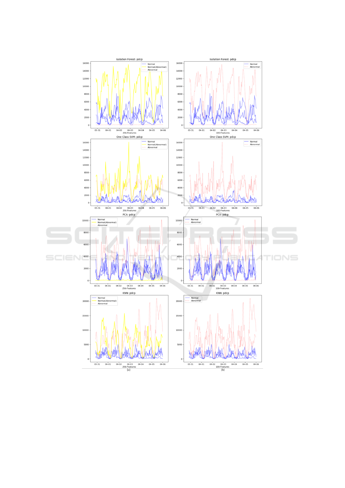
Figure 7: Comparison of detection results before and after feature selection. Figure (a) is the detection result obtained by

training an unsupervised model based on 256-dimensional original features, and Figure (b) is an abnormal wireless network

cell detected using 100-dimensional important features. From top to bottom, the detection results of Isolation Forest, One

Class SVM, PCA, and KNN are selected. Each ﬁgure selected the PDCP indicators of multiple wireless network cells

for display. The abscissa represents the time series point, and the ordinate represents the indicator value. The red legend

represents the detected abnormal wireless network cell, the blue is the normal, and the yellow represents the abnormal data

but the algorithm does not detect the situation (the algorithm judges the normal wireless network cell).

Research on Optimization of 4G-LTE Wireless Network Cells Anomaly Diagnosis Algorithm based on Multidimensional Time Series Data

Table 8: Important features set.

Indicator Fields Statistical Features

pdcp

kpi, last hour, max, mean, med, min, samehour max,

samehour mean, samehour med, samehour min, samehour std, std

Radio InitSuccConn Rate kpi, last hour, min, samehour max, samehour mean

S1Sig FailConnEstab kpi, mean, samehour med, samehour min

RRC FailConnEstab last hour, std

ERAB FailEstab kpi, mean, samehour mean, std

UECNTX AbnormRel kpi, last hour, mean, med, std

UECNTX Drop Rate kpi, med, samehour mean, samehour med

ERAB AbnormRel kpi, last hour, mean, samehour mean

ERAB Drop Rate med

RRC ConnReestab Rate kpi, last hour, mean, med, samehour max, samehour min

RRC AttConnReestab max, mean, samehour mean, samehour med

HO SuccOutIntraFreq Rate kpi, last hour, min, samehour min, samehour std, std

HO FailOutIntraFreq kpi, last hour, samehour med

HO FailOutInterFreq kpi, med, samehour med, samehour min

cqi rate kpi, last hour, samehour max, samehour min, samehour std

phy rrurxrssimean chan1

kpi, last hour, min, samehour max, samehour mean,

samehour med, samehour std, std

PDCP SduLossPktUl Rate kpi, samehour max, samehour mean

PDCP SduLossPktDl kpi, last hour, samehour max, samehour std

PDCP SduLossPktDl Rate kpi, samehour min, samehour std

PDCP SduDiscardPktDl Rate

kpi, last hour, max, mean, med, samehour max,

samehour mean, samehour med, samehour min, samehour std, std

hours hours

day of the week day of the week

Table 9: Comparison of evaluation indicators before and

after feature selection.

Algorithm Eval

256-D

(%)

100-D

(%)

Inc (%)

Isolation

Forest

Accuracy 98.5 98.7 +0.2

Recall 11.0 27.5 +16.5

F1-Score 8.2 20.5 +12.3

AUC 55.0 63.3 +8.3

OneClass-

SVM

Accuracy 96.7 97.5 +0.8

Recall 23.4 30.3 +6.9

F1-Score 8.2 12.5 +4.3

AUC 60.3 64.1 +3.8

PCA

Accuracy 98.5 98.6 +0.1

Recall 8.4 20.5 +12.1

F1-Score 6.2 15.3 +9.1

AUC 53.7 59.8 +6.1

KNN

Accuracy 98.6 98.7 +0.1

Recall 11.1 16.2 +5.1

F1-Score 8.5 12.6 +4.1

AUC 55.1 57.7 +2.6

Ensemble

algorithms

Accuracy - 98.3 -

Recall - 31.1 -

F1-Score - 17.7 -

AUC - 64.9 -

can be weighted and fused, and the Recall index af-

ter fusion is increased by 3.6%, and more abnormal

wireless network cells can be detected after the fu-

sion. In summary, the effect of constructing a fea-

ture set on the original data and performing anomaly

detection through an unsupervised algorithm is rela-

tively poor, while the detection effect of the same al-

gorithm on the feature set after feature screening has

been greatly improved. The meaning of this paper

mainly includes two aspects. On the one hand, in

the massive unlabeled data, building important fea-

ture sets through small samples of labeled data and

supervised algorithms can assist the training of un-

supervised algorithms, thereby improving the detec-

tion performance of unsupervised algorithms. On the

other hand, through the optimization training of unsu-

pervised algorithm, a large amount of data can be pre-

annotated to provide an auxiliary decision-making

role for the follow-up annotation work of experts.

In the future work, we will try to unify the opin-

ions of different operation and maintenance engineers

as much as possible to obtain higher quality annota-

tion results. Although the evaluation indicators of this

article have been improved, the current inconsisten-

cies in the annotations have caused the ﬁnal recall to

be unsatisfactory, and this experiment only selected

4G-LTE wireless network cell data in a few regions.

In the future, we will use data from more provinces

for optimization and veriﬁcation to better improve the

current wireless network base station operation and

maintenance methods.

IoTBDS 2021 - 6th International Conference on Internet of Things, Big Data and Security

REFERENCES

Aggarwal, C. C. (2015). Outlier analysis. In Data mining,

pages 237–263. Springer.

Angiulli, F. and Pizzuti, C. (2002). Fast outlier detection in

high dimensional spaces. In European conference on

principles of data mining and knowledge discovery,

pages 15–27. Springer.

Aryal, S., Ting, K. M., Wells, J. R., and Washio, T. (2014).

Improving iforest with relative mass. In Paciﬁc-Asia

Conference on Knowledge Discovery and Data Min-

ing, pages 510–521. Springer.

Bai, S., Kolter, J. Z., and Koltun, V. (2018). An em-

pirical evaluation of generic convolutional and recur-

rent networks for sequence modeling. arXiv preprint

arXiv:1803.01271.

Buckland, M. and Gey, F. (1994). The relationship between

recall and precision. Journal of the American society

for information science, 45(1):12–19.

Chandola, V., Banerjee, A., and Kumar, V. (2009).

Anomaly detection: A survey. ACM computing sur-

veys (CSUR), 41(3):1–58.

Chawla, N. V., Bowyer, K. W., Hall, L. O., and Kegelmeyer,

W. P. (2002). Smote: synthetic minority over-

sampling technique. Journal of artiﬁcial intelligence

research, 16:321–357.

Chen, M., Liu, Q., Chen, S., Liu, Y., Zhang, C.-H., and

Liu, R. (2019). Xgboost-based algorithm interpre-

tation and application on post-fault transient stabil-

ity status prediction of power system. IEEE Access,

7:13149–13158.

Chen, T. and Guestrin, C. (2016). Xgboost: A scalable

tree boosting system. In Proceedings of the 22nd acm

sigkdd international conference on knowledge discov-

ery and data mining, pages 785–794.

George, A. and Vidyapeetham, A. (2012). Anomaly detec-

tion based on machine learning dimensionality reduc-

tion using pca and classiﬁcation using svm. Interna-

tional Journal of Computer Applications, 47(21):5–8.

Hastie, T., Tibshirani, R., and Friedman, J. (2009). The el-

ements of statistical learning: data mining, inference,

and prediction. Springer Science & Business Media.

Kim, J. and Scott, C. D. (2012). Robust kernel density esti-

mation. The Journal of Machine Learning Research,

13(1):2529–2565.

Kleinbaum, D. G., Dietz, K., Gail, M., Klein, M., and Klein,

M. (2002). Logistic regression. Springer.

Lee Rodgers, J. and Nicewander, W. A. (1988). Thirteen

ways to look at the correlation coefﬁcient. The Amer-

ican Statistician, 42(1):59–66.

Pradhan, M., Pradhan, S. K., and Sahu, S. K. (2012).

Anomaly detection using artiﬁcial neural network.

International Journal of Engineering Sciences &

Emerging Technologies, 2(1):29–36.

Shyu, M.-L., Chen, S.-C., Sarinnapakorn, K., and Chang,

L. (2003). A novel anomaly detection scheme based

on principal component classiﬁer. Technical report,

Miami Univ Coral Gables FL Dept of Electrical and

Computer Engineering.

Sokolova, M., Japkowicz, N., and Szpakowicz, S. (2006).

Beyond accuracy, f-score and roc: a family of discrim-

inant measures for performance evaluation. In Aus-

tralasian joint conference on artiﬁcial intelligence,

pages 1015–1021. Springer.

Walter, S. D. (2005). The partial area under the summary

roc curve. Statistics in medicine, 24(13):2025–2040.

Wang, Y., Wong, J., and Miner, A. (2004). Anomaly in-

trusion detection using one class svm. In Proceedings

from the Fifth Annual IEEE SMC Information Assur-

ance Workshop, 2004., pages 358–364. IEEE.

Wazid, M. and Das, A. K. (2016). An efﬁcient hybrid

anomaly detection scheme using k-means clustering

for wireless sensor networks. Wireless Personal Com-

munications, 90(4):1971–2000.

Research on Optimization of 4G-LTE Wireless Network Cells Anomaly Diagnosis Algorithm based on Multidimensional Time Series Data